Genome: Difference between revisions
| (629 intermediate revisions by the same user not shown) | |||
| Line 1: | Line 1: | ||
= Visualization = | = Visualization = | ||
* [https://github.com/cmdcolin/awesome-genome-visualization Awesome genome visualization] | |||
* [http://www.bioconductor.org/packages/release/BiocViews.html#___Visualization Bioconductor > BiocViews > Visualization]. Search 'genom' as the keyword. | |||
== Ten simple rules == | |||
[https://journals.plos.org/ploscompbiol/article?id=10.1371%2Fjournal.pcbi.1010622 Ten simple rules for developing visualization tools in genomics] | |||
== [http://software.broadinstitute.org/software/igv/ IGV] == | == [http://software.broadinstitute.org/software/igv/ IGV] == | ||
| Line 37: | Line 41: | ||
* DNA: no matter it is whole genome or whole exome, the coverage is more even. For whole exome, there is no splicing. | * DNA: no matter it is whole genome or whole exome, the coverage is more even. For whole exome, there is no splicing. | ||
* RNA: focusing on expression so the coverage changes a lot. The base name still A,C,G,T (not A,C,G,U). | * RNA: focusing on expression so the coverage changes a lot. The base name still A,C,G,T (not A,C,G,U). | ||
=== ChromoMap === | |||
[https://bmcbioinformatics.biomedcentral.com/articles/10.1186/s12859-021-04556-z ChromoMap]: an R package for interactive visualization of multi-omics data and annotation of chromosomes | |||
== RNA-seq DRaMA == | |||
https://hssgenomics.shinyapps.io/RNAseq_DRaMA/ from [https://blog.rstudio.com/2020/07/13/winners-of-the-2nd-shiny-contest/ 2nd Annual Shiny Contest] | |||
== [http://www.bioconductor.org/packages/release/bioc/html/Gviz.html Gviz] == | == [http://www.bioconductor.org/packages/release/bioc/html/Gviz.html Gviz] == | ||
| Line 47: | Line 57: | ||
== [http://www.bioconductor.org/packages/release/bioc/html/ggbio.html ggbio] == | == [http://www.bioconductor.org/packages/release/bioc/html/ggbio.html ggbio] == | ||
[https://support.bioconductor.org/p/9152800/ Wondering how to look at the reads of a gene in samples to check if it was knocked out?] | |||
== [http://www.bioconductor.org/packages/release/bioc/html/NOISeq.html NOISeq] package == | == [http://www.bioconductor.org/packages/release/bioc/html/NOISeq.html NOISeq] package == | ||
| Line 62: | Line 73: | ||
See fig on p22 of [http://www.bioconductor.org/packages/release/bioc/vignettes/Sushi/inst/doc/Sushi.pdf Sushi vignette] where genes with different strands are shown with different directions when plotGenes() was used. plotGenes() can be used to plot gene structures that are stored in bed format. | See fig on p22 of [http://www.bioconductor.org/packages/release/bioc/vignettes/Sushi/inst/doc/Sushi.pdf Sushi vignette] where genes with different strands are shown with different directions when plotGenes() was used. plotGenes() can be used to plot gene structures that are stored in bed format. | ||
== [http://www.cbioportal.org/ cBioPortal] | == [http://www.cbioportal.org/ cBioPortal], TCGA, PanCanAtlas == | ||
See [[Tcga|TCGA]]. | |||
== TCPA == | |||
[https://www.tcpaportal.org/tcpa/download.html Download]. Level 4. | |||
[https://www. | |||
== [http://qualimap.bioinfo.cipf.es/ Qualimap] == | == [http://qualimap.bioinfo.cipf.es/ Qualimap] == | ||
| Line 74: | Line 84: | ||
== [http://www.bioinformatics.babraham.ac.uk/projects/seqmonk/ SeqMonk] == | == [http://www.bioinformatics.babraham.ac.uk/projects/seqmonk/ SeqMonk] == | ||
SeqMonk is a program to enable the visualisation and analysis of mapped sequence data. | SeqMonk is a program to enable the visualisation and analysis of mapped sequence data. | ||
== dittoSeq == | |||
[https://rna-seqblog.com/dittoseq-universal-user-friendly-single-cell-and-bulk-rna-sequencing-visualization-toolkit-bioinformatics/ dittoSeq] – universal user-friendly single-cell and bulk RNA sequencing visualization toolkit, bioinformatics | |||
== SeqCVIBE == | |||
[https://www.rna-seqblog.com/seqcvibe-interactive-analysis-exploration-and-visualization-of-rna-seq-data/ SeqCVIBE – interactive analysis, exploration, and visualization of RNA-Seq data] | |||
== ggcoverage == | |||
[https://bmcbioinformatics.biomedcentral.com/articles/10.1186/s12859-023-05438-2 ggcoverage: an R package to visualize and annotate genome coverage for various NGS data] 2023 | |||
= Copy Number = | = Copy Number = | ||
| Line 103: | Line 122: | ||
== modSaRa2 == | == modSaRa2 == | ||
[https://academic.oup.com/bioinformatics/article/35/17/2891/5288773 An accurate and powerful method for copy number variation detection] | [https://academic.oup.com/bioinformatics/article/35/17/2891/5288773 An accurate and powerful method for copy number variation detection] | ||
== Visualization == | |||
[https://academic.oup.com/bioinformatics/article/37/8/1164/5895301 reconCNV: interactive visualization of copy number data from high-throughput sequencing] 2021 | |||
= NGS = | = NGS = | ||
[[:File:CentralDogmaMolecular.png]] | [[:File:CentralDogmaMolecular.png]] | ||
See [[NGS|NGS]]. | |||
== mNGS == | |||
[https://www.top1health.com/Article/93836 找出病原菌的新武器 :總基因體次世代定序是什麼?] | |||
=== RNA- | = R and Bioconductor packages = | ||
== Resources == | |||
* [https://cran.r-project.org/web/views/Omics.html CRAN Task View: Genomics, Proteomics, Metabolomics, Transcriptomics, and Other Omics] | |||
* [http://rafalab.github.io/pages/harvardx.html HarvardX Biomedical Data Science Open Online Training], [https://hbctraining.github.io/main/ Bioinformatics Training at the Harvard Chan Bioinformatics Core] | |||
* [https://liulab-dfci.github.io/bioinfo-combio/ Introduction to Bioinformatics and Computational Biology] Xiaole Shirley Liu (ebook & videos) | |||
* [https://bioconductor.org/help/course-materials/2017/CSAMA/ CSAMA 2017: Statistical Data Analysis for Genome-Scale Biology] | |||
* [https://nsaunders.wordpress.com/2015/04/28/some-basics-of-biomart/ Some basics of biomaRt] (and GenomicRanges) | |||
* [http://master.bioconductor.org/help/workflows/annotation/AnnotatingRanges/ Annotating Ranges] Represent common sequence data types (e.g., from BAM, gff, bed, and wig files) as genomic ranges for simple and advanced range-based queries. | |||
<pre> | |||
library(VariantAnnotation) | |||
library(AnnotationHub) | |||
library(TxDb.Hsapiens.UCSC.hg19.knownGene) | |||
library(TxDb.Mmusculus.UCSC.mm10.ensGene) | |||
library(org.Hs.eg.db) | |||
library(org.Mm.eg.db) | |||
library(BSgenome.Hsapiens.UCSC.hg19) | |||
</pre> | |||
* [http://faculty.ucr.edu/~tgirke/HTML_Presentations/Manuals/Workshop_Dec_6_10_2012/Rrnaseq/Rrnaseq.pdf Analysis of RNA-Seq Data with R/Bioconductor] by Girke in UC Riverside | |||
* [http://ivory.idyll.org/dibsi/index.html 2018 Data Intensive Biology Summer Institute at UC Davis] | |||
* [http://www.ebi.ac.uk/training/sites/ebi.ac.uk.training/files/materials/2012/121029_HTS/martin_morgan1_nicolas_delhomme2_embo2012_rbioconductor.pdf R / Bioconductor for High-Throughput Sequence Analysis 2012] by Martin Morgan1 and Nicolas Delhomme | |||
* [http://www-huber.embl.de/pub/pdf/nprot.2013.099.pdf Count-based differential expression analysis of RNA sequencing data using R and Bioconductor] by Simon Anders | |||
* [http://www.ebi.ac.uk/training/sites/ebi.ac.uk.training/files/materials/2013/131021_HTS/genesandgenomes.pdf Sequences, Genomes, and Genes in R / Bioconductor] by Martin Morgan 2013. | |||
* [http://www.ncbi.nlm.nih.gov/pmc/articles/PMC4509590/ Orchestrating high-throughput genomic analysis with Bioconductor] by Wolfgang Huber et al 2015. | |||
* [https://rpubs.com/achitsaz/97976 RNA-seq Analysis Example] This is a script that will do differential gene expression (DGE) analysis for RNA-seq experiments using the bioconductor package edgeR. RPKMs were calculated for bar plots. | |||
* [https://github.com/pgpmartin/BioC_For_NGS/blob/master/BioC_for_NGS_PMartin.pdf An introduction to R and Bioconductor for the analysis of high-throughput sequencing data] by Pascal MARTIN Oct 2018 | |||
* [https://morphoscape.wordpress.com/2022/07/28/bioinformatics-analysis-of-omics-data-with-the-shell-r/ Bioinformatics Analysis of Omics Data with the Shell & R] | |||
=== | === Docker === | ||
https:// | [https://github.com/jhuanglab/bioinstaller Bioinstaller]: A comprehensive R package to construct interactive and reproducible biological data analysis applications based on the R platform. Package on [https://cran.r-project.org/web/packages/BioInstaller/ CRAN]. | ||
=== RNA-Seq | == Some workflows == | ||
* | === RNA-Seq workflow === | ||
* | Gene-level exploratory analysis and differential expression. A non stranded-specific and paired-end rna-seq experiment was used for the tutorial. | ||
<pre> | |||
STAR Samtools Rsamtools | |||
fastq -----> sam ----------> bam ----------> bamfiles -| | |||
\ GenomicAlignments DESeq2 | |||
--------------------> se --------> dds | |||
GenomicFeatures GenomicFeatures / (SummarizedExperiment) (DESeqDataSet) | |||
gtf ----------------> txdb ---------------> genes -----| | |||
</pre> | |||
* https://bioconductor.org/packages/3.12/workflows/ | |||
* [http://www.bioconductor.org/help/workflows/rnaseqGene/ RNA-Seq workflow] | |||
* [https://www.bioconductor.org/packages/release/workflows/html/RnaSeqGeneEdgeRQL.html RnaSeqGeneEdgeRQL] | |||
* [http://www.sthda.com/english/wiki/rna-seq-differential-expression-work-flow-using-deseq2 RNA-Seq differential expression work flow using DESeq2] | |||
* [https://docs.gdc.cancer.gov/Data/Bioinformatics_Pipelines/Expression_mRNA_Pipeline/ mRNA Analysis Pipeline] from NIC GDC | |||
=== | === rnaseqGene === | ||
[http://master.bioconductor.org/packages/release/workflows/html/rnaseqGene.html rnaseqGene] - RNA-seq workflow: gene-level exploratory analysis and differential expression | |||
[http://master.bioconductor.org/packages/release/bioc/html/tximport.html tximport] | |||
[https://codeocean.com/capsule/2296412/tree/v1 CodeOcean] - Differential analyses for RNA-seq: transcript-level estimates improve gene-level inferences (version: 1.17.5). [https://codeocean.com/pricing Plan]. | |||
=== | === [http://master.bioconductor.org/help/workflows/high-throughput-sequencing/ Sequence analysis] === | ||
<pre> | |||
library(ShortRead) or library(Biostrings) (QA) | |||
gtf + library(GenomicFeatures) or directly library(TxDb.Scerevisiae.UCSC.sacCer2.sgdGene) (gene information) | |||
GenomicRanges::summarizeOverlaps or GenomicRanges::countOverlaps(count) | |||
edgeR or DESeq2 (gene expression analysis) | |||
library(org.Sc.sgd.db) or library(biomaRt) | |||
</pre> | |||
== | === [http://master.bioconductor.org/help/workflows/annotation/annotation/ Accessing Annotation Data] === | ||
Use microarray probe, gene, pathway, gene ontology, homology and other annotations. Access GO, KEGG, NCBI, Biomart, UCSC, vendor, and other sources. | |||
<source lang="rsplus"> | |||
library(org.Hs.eg.db) # Sample OrgDb Workflow | |||
library("hgu95av2.db") # Sample ChipDb Workflow | |||
library(TxDb.Hsapiens.UCSC.hg19.knownGene) # Sample TxDb Workflow | |||
library(Homo.sapiens) # Sample OrganismDb Workflow | |||
library(AnnotationHub) # Sample AnnotationHub Workflow | |||
library("biomaRt") # Using biomaRt | |||
library(BSgenome.Hsapiens.UCSC.hg19) # BSgenome packages | |||
</source> | |||
= | {| class="wikitable" | ||
! Object type | |||
! example package name | |||
! contents | |||
|- | |||
| OrgDb | |||
| org.Hs.eg.db | |||
| gene based information for Homo sapiens | |||
|- | |||
| TxDb | |||
| TxDb.Hsapiens.UCSC.hg19.knownGene | |||
| transcriptome ranges for Homo sapiens | |||
|- | |||
| OrganismDb | |||
| Homo.sapiens | |||
| composite information for Homo sapiens | |||
|- | |||
| BSgenome | |||
| BSgenome.Hsapiens.UCSC.hg19 | |||
| genome sequence for Homo sapiens | |||
|- | |||
| | |||
| [http://cran.r-project.org/web/packages/refGenome/index.html refGenome] | |||
| | |||
|} | |||
* | == RNA-Seq Data Analysis using R/Bioconductor == | ||
* | * https://github.com/datacarpentry/rnaseq-data-analysis by Stephen Turner. | ||
* | * [https://support.bioconductor.org/p/69677/ Tutorial: Introduction to Bioconductor for high-throughput sequence analysis] by UseR 2015 | ||
* [http://bioconductor.org/packages/release/bioc/html/systemPipeR.html systemPipeR] Building end-to-end analysis pipelines with automated report generation for next generation sequence (NGS) applications such as RNA-Seq, ChIP-Seq, VAR-Seq and Ribo-Seq. An important feature is support for running command-line software, such as NGS aligners, on both single machines or compute clusters. | |||
** http://girke.bioinformatics.ucr.edu/GEN242/mydoc_systemPipeVARseq_05.html | |||
* [http://bioconductor.org/help/course-materials/2015/BioC2015/ BioC2015] | |||
=== | === recount2 === | ||
* https://github.com/leekgroup/recount | |||
* [https://jhubiostatistics.shinyapps.io/recount/ recount2] - A multi-experiment resource of analysis-ready RNA-seq gene and exon count datasets. | |||
* [https://github.com/LieberInstitute/recountWorkshop2020 Human RNA-seq data from recount2 and related packages] from [https://bioc2020.bioconductor.org/workshops BioC 2020 Workshop] | |||
** recount2 works with DESeq2, edgeR and limma-voom | |||
=== [ | === recount3 === | ||
* [https://lcolladotor-github-io.translate.goog/rnaseq_LCG-UNAM_2022/datos-de-rna-seq-a-trav%C3%A9s-de-recount3.html?_x_tr_sl=auto&_x_tr_tl=en&_x_tr_hl=en&_x_tr_pto=wapp Intro RNA-seq LCG-UNAM 2022] (Spanish) | |||
* [https://support.bioconductor.org/p/9152538/ Recount3: PCR duplicates]. | |||
** [https://www.khanacademy.org/science/ap-biology/gene-expression-and-regulation/biotechnology/a/polymerase-chain-reaction-pcr PCR duplication] can refer to two different things. It can mean the process of making many copies of a specific DNA region using a technique called Polymerase Chain Reaction (PCR). PCR relies on a thermostable DNA polymerase and requires DNA primers designed specifically for the DNA region of interest. | |||
** On the other hand, [https://www.nature.com/articles/nmeth.4268 PCR duplication] can also refer to a problem that occurs when the same DNA fragment is amplified and sequenced multiple times, resulting in identical reads that can bias many types of high-throughput-sequencing experiments. These identical reads are called [https://bmcgenomics.biomedcentral.com/articles/10.1186/s12864-018-4933-1 PCR duplicates] and can be eliminated using various methods such as removing all but one read of identical sequences or using '''unique molecular identifiers (UMIs)''' to enable accurate counting and tracking of molecules. | |||
** '''UMI''' stands for Unique Molecular Identifier. [https://dnatech.genomecenter.ucdavis.edu/faqs/what-are-umis-and-why-are-they-used-in-high-throughput-sequencing/ It is a complex index added to sequencing libraries before any PCR amplification steps, enabling the accurate bioinformatic identification of PCR duplicates]. UMIs are also known as '''Molecular Barcodes''' or '''Random Barcodes'''. UMIs are valuable tools for both quantitative sequencing applications and also for genomic variant detection, especially the detection of rare mutations. UMI sequence information in conjunction with alignment coordinates enables grouping of sequencing data into read families representing individual sample DNA or RNA fragments. | |||
** [https://umi-tools.readthedocs.io/en/latest/reference/dedup.html '''dedup'''] - Deduplicate reads using UMI and mapping coordinates | |||
** UMIs can be extracted from a fastq file using awk. For example '''awk 'NR % 4 == 1 {split($0,a,":"); print a[6]}' input.fastq > umis.txt''' . Here we assume the read header is '''@SEQ_ID:LANE:TILE:X:Y:UMI, then the UMI sequence is in the 6th field, following the 5th colon.''' | |||
== dbGap == | |||
[https://academic.oup.com/bioinformatics/article/36/4/1305/5556117 dbgap2x: an R package to explore and extract data from the database of Genotypes and Phenotypes (dbGaP)] | |||
=== [ | == eQTL == | ||
https:// | [https://www.coursera.org/lecture/statistical-genomics/combining-data-types-eqtl-6-04-NkorV Statistics for Genomic Data Science] (Coursera) and [https://cran.r-project.org/web/packages/MatrixEQTL/index.html MatrixEQTL] from CRAN | ||
== [https://bioconductor.org/packages/release/bioc/html/GenomicDataCommons.html GenomicDataCommons] package == | |||
https:// | * Genomic Data Commons | ||
** https://gdc.cancer.gov/ | |||
** https://www.cancer.gov/about-nci/organization/ccg/research/computational-genomics/gdc | |||
** [https://portal.gdc.cancer.gov/ Data Portal]. A list of [https://portal.gdc.cancer.gov/projects Projects] | |||
* Use the GenomicDataCommons package to find and download variants from TCGA (NCI Genomic Data Commons Access) dataset and maftools package for analysis and visualization. See https://seandavi.github.io/talk/2018/02/08/bioconductor-a-potential-hub-in-the-cancer-biomarker-data-ecosystem/ | |||
* https://seandavi.github.io/post/2018/03/extracting-clinical-information-using-the-genomicdatacommons-package/ | |||
* [https://docs.google.com/presentation/d/1bjnW67aemW90kFcq_S5rGorX96Xjrp9jt3tM4PpNuHI The Cancer Data Ecosystem: Data and cloud resources for cancer data science] | |||
* [https://docs.google.com/presentation/d/1z0fgKWQrshn9rB2HJ4oiNd4V2tZUeomvre4p3usw6hc The GenomicDataCommons and GEOquery Bioconductor Packages] | |||
Note: | |||
# The TCGA data such as [https://portal.gdc.cancer.gov/projects/TCGA-LUAD TCGA-LUAD] are not part of clinical trials (described [https://wiki.cancerimagingarchive.net/display/Public/TCGA-LUAD here]). | |||
# Each patient has 4 categories data and the 'case_id' is common to them: | |||
#* demographic: gender, race, year_of_birth, year_of_death | |||
#* diagnoses: tumor_stage, age_at_diagnosis, tumor_grade | |||
#* exposures: cigarettes_per_day, alcohol_history, years_smoked, bmi, alcohol_intensity, weight, height | |||
#* main: disease_type, primary_site | |||
# The original download (clinical.tsv file) data contains a column 'treatment_or_therapy' but it has missing values for all patients. | |||
=== | == Visualization == | ||
[https:// | === [https://bioconductor.org/packages/release/bioc/html/GenVisR.html GenVisR] === | ||
== | === [http://www.bioconductor.org/packages/devel/bioc/html/ComplexHeatmap.html ComplexHeatmap] === | ||
=== | == Read counts == | ||
[[ | === Read, fragment === | ||
* [https://biology.stackexchange.com/a/30150 Meaning of the "reads" keyword in terms of RNA-seq or next generation sequencing]. A read refers to the sequence of a cluster that is obtained after the end of the sequencing process which is ultimately the sequence of a section of a unique fragment. | |||
* [https://www.biostars.org/p/106291/ What is the difference between a Read and a Fragment in RNA-seq?]. Diagram , Pair-end, single-end. | |||
* In the context of RNA-seq, "read" and "fragment" may refer to slightly different things, but they are related concepts. | |||
** A '''read''' is a short sequence of nucleotides that has been generated by a sequencing machine. These reads are typically around 100-150 bases long. RNA-seq experiments generate millions or billions of reads, and these reads are aligned to a reference genome or transcriptome to determine which reads came from which genes or transcripts, this information is used to quantify gene and transcript expression levels. | |||
** A '''fragment''' is a piece of RNA that has been broken up and converted into a read. In RNA-seq, the first step is to convert the RNA into a library of fragments. To do this, the RNA is typically broken up into smaller pieces using a process called fragmentation. Then, '''adapters''' are added to the ends of the fragments to allow them to be sequenced. The fragments are then converted into a library of reads that can be sequenced using a next-generation sequencing platform. | |||
** In summary, a read is a short sequence of nucleotides that has been generated by a sequencing machine, whereas a fragment is a piece of RNA that has been broken up and converted into a read. The process of fragmentation creates a library of fragments that are then converted into reads that can be sequenced. | |||
* Does one fragment contain 1 read or multiple reads? | |||
** One fragment in RNA-seq can contain multiple reads, depending on the sequencing technology and library preparation protocol used. | |||
** In the process of library preparation, RNA is first fragmented into smaller pieces, then adapters are ligated to the ends of the fragments. The fragments are then amplified using PCR, generating multiple copies of the original fragment. These amplified fragments are then sequenced using a next-generation sequencing platform, generating multiple reads per fragment. | |||
** For example, in '''Illumina''' sequencing, fragments are ligated with adapters, then they are clonally amplified using bridge amplification. This allows for the creation of '''clusters''' of identical copies of the original fragment on a sequencing flow cell. Then, each '''cluster''' is sequenced, generating a large number of reads per fragment. | |||
** In other technologies like '''PacBio''' or '''Nanopore''', the sequencing of a fragment generates only one read, as the technology can read long stretches of DNA, therefore it doesn't need to fragment the RNA prior to sequencing. | |||
** In summary, one fragment in RNA-seq can contain multiple reads, depending on the sequencing technology and library preparation protocol used. '''The number of reads per fragment can vary from one to several thousands.''' | |||
* How many reads in a fragment on average in illumination sequencing? | |||
** The number of reads per fragment in Illumina sequencing can vary depending on the sequencing platform and library preparation protocol used, as well as the sequencing depth and the complexity of the sample. However, on average, one fragment can generate several hundred to several thousand reads in Illumina sequencing. | |||
** When sequencing is performed on the Illumina platform, the process of library preparation includes fragmenting the RNA into smaller pieces, ligating adapters to the ends of the fragments, and then amplifying the fragments using bridge amplification. This allows for the creation of clusters of identical copies of the original fragment on a sequencing flow cell. Then, each cluster is sequenced, generating multiple reads per fragment. | |||
** The number of reads per fragment can also be affected by the sequencing depth, which refers to the total number of reads generated by the sequencing machine. A higher sequencing depth will result in more reads per fragment, while a lower sequencing depth will result in fewer reads per fragment. | |||
** In summary, the number of reads per fragment in Illumina sequencing can vary, but on average, one fragment can generate several hundred to several thousand reads. The number of reads per fragment can be influenced by the sequencing platform, library preparation protocol, sequencing depth, and the complexity of the sample. | |||
=== [http://bioconductor.org/packages/release/bioc/html/Rsubread.html Rsubread] === | |||
* See [https://support.bioconductor.org/p/65604/ this post] for about C version of the [http://bioinf.wehi.edu.au/featureCounts/ featureCounts] program. | |||
* [https://www.biostars.org/p/96176/ featureCounts vs HTSeq-count] | |||
* [http://bioinformatics.cvr.ac.uk/blog/featurecounts-or-htseq-count/ featureCounts or htseq-count?] | |||
* [https://www.jianshu.com/p/9cc4e8657d62 featurecounts的使用说明] | |||
* [https://www.ncbi.nlm.nih.gov/geo/query/acc.cgi?acc=GSE62944 GSE62944] TCGA data processed by Rahman M. | |||
=== RSEM === | |||
<ul> | |||
<li>[http://deweylab.github.io/RSEM/ RSEM], [https://deweylab.github.io/RSEM/rsem-calculate-expression.html rsem-calculate-expression] </li> | |||
<li>[https://hpc.nih.gov/apps/rsem.html RSEM on Biowulf] | |||
<syntaxhighlight lang='sh'> | |||
$ mkdir SeqTestdata/RNASeqFibroblast/output | |||
$ sinteractive --cpus-per-task=2 --mem=10g | |||
$ module load rsem bowtie STAR | |||
$ rsem-calculate-expression -p 2 --paired-end --star \ | |||
../test.SRR493366_1.fastq ../test.SRR493366_2.fastq \ | |||
/fdb/rsem/ref_from_genome/hg19 Sample1 # 12 seconds | |||
$ ls -lthog | |||
total 5.8M | |||
-rw-r----- 1 1.6M Nov 24 13:39 Sample1.genes.results | |||
-rw-r----- 1 2.5M Nov 24 13:39 Sample1.isoforms.results | |||
-rw-r----- 1 1.6M Nov 24 13:39 Sample1.transcript.bam | |||
drwxr-x--- 2 4.0K Nov 24 13:39 Sample1.stat | |||
$ wc -l Sample1.genes.results | |||
26335 Sample1.genes.results | |||
$ wc -l Sample1.isoforms.results | |||
51399 Sample1.isoforms.results | |||
2. | $ head -2 Sample1.genes.results | ||
gene_id transcript_id(s) length effective_length expected_count TPM FPKM | |||
A1BG NM_130786 1766.00 1589.99 0.00 0.00 0.00 | |||
$ head -2 Sample1.isoforms.results | |||
transcript_id gene_id length effective_length expected_count TPM FPKM IsoPct | |||
NM_130786 A1BG 1766 1589.99 0.00 0.00 0.00 0.00 | |||
</ | $ head -1 /fdb/rsem/ref_from_genome/hg19.transcripts.fa | ||
>NM_130786 | |||
$ grep NM_130786 /fdb/igenomes/Homo_sapiens/UCSC/hg19/transcriptInfo.tab | |||
NM_130786 2721192635 2721199328 2721188175 2 8 431185 | |||
</syntaxhighlight> | |||
</li> | |||
</ul> | |||
* [http://cshprotocols.cshlp.org/content/2019/6/pdb.prot098368.full An RNA-Seq Protocol for Differential Expression Analysis] Owens 2019 | |||
* [https://www.cbioportal.org/ Cbioportal] -> [https://www.cbioportal.org/study/summary?id=brca_tcga_pan_can_atlas_2018 Breast Invasive Carcinoma (TCGA, PanCancer Atlas)] -> Explore selected study -> Original data -> [https://gdc.cancer.gov/about-data/publications/pancanatlas PanCanAtlas Publications] -> RNA (Final) - EBPlusPlusAdjustPANCAN_IlluminaHiSeq_RNASeqV2.geneExp.tsv | |||
* [https://bmcgenomics.biomedcentral.com/articles/10.1186/s12864-017-4002-1 Evaluation and comparison of computational tools for RNA-seq isoform quantification] 2017 | |||
* [https://www.rna-seqblog.com/the-concepts-of-mean-fragment-length-and-effective-length-in-rna-sequencing/ The Concepts of Mean Fragment Length and Effective Length in RNA Sequencing] | |||
<ul> | |||
<li>RSEM gene level result file (see [[#tximport|here for an example]]) contains 5 essential columns (and the element saved by '''tximport'''() function) excluding transcript_id | |||
<ul> | |||
<li>[https://groups.google.com/g/rsem-users/c/IaZmviqghJc Effective length] → length. This is different across samples. This is much shorter than Length (e.g. 105 vs 1). </li> | |||
<li>[http://deweylab.biostat.wisc.edu/rsem/rsem-calculate-expression.html Expected count] → count. This is the sum of the posterior probability of each read comes from this transcript over all reads. </li> | |||
<li>TPM → abundance. The sum of all transcripts' TPM is 1 million. </li> | |||
<li>FPKM (not kept?). FPKM_i = 10^3 / l_bar * TPM_i for gene i. So for each sample FPKM is a scaling of TPM. </li> | |||
</ul> | |||
<pre> | <pre> | ||
R> dfpkm[1:5, 1:3] / txi.rsem$abundance[1:5, 1:3] | |||
144126_210-T_JKQFX5 144126_210-T_JKQFX6 144126_210-T_JKQFX8 | |||
5S_rRNA 0.7563603 1.118008 0.8485292 | |||
5_8S_rRNA NaN NaN NaN | |||
6M1-18 NaN NaN NaN | |||
7M1-2 NaN NaN NaN | |||
7SK 0.7563751 1.118029 0.8485281 | |||
</pre> | </pre> | ||
<li>An example using [https://www.rdocumentation.org/packages/tximport/versions/1.0.3/topics/tximport tximport::tximport()] and [https://www.rdocumentation.org/packages/DESeq2/versions/1.12.3/topics/DESeqDataSet-class DESeq2::DESeqDataSetFromTximport]. <span style="color: red">Note it directly uses round(expected_count) to get the integer-value counts.</span> See the source of DESeqDataSetFromTximport() [https://github.com/mikelove/DESeq2/blob/6aa81f9906e192eea1fb21cdc492b26ee4a472f1/R/AllClasses.R#L405 here]. The [https://bioconductor.org/packages/release/bioc/vignettes/tximport/inst/doc/tximport.html tximport vignette] has discussed two suggested ways of importing estimates for use with differential gene expression (DGE) methods in the section of "Downstream DGE in Bioconductor". The vignette does not say anything about "expected_count" from RSEM output. | |||
The two | |||
<pre> | <pre> | ||
txi.rsem <- tximport(files, type = "rsem", txIn = F, txOut = F) | |||
txi.rsem$length[txi.rsem$length == 0] <- 1 | |||
names(txi.rsem) # a list, | |||
# length = effective_length (matrix) | |||
# counts = expected counts column (matrix), non-integer | |||
# abundance = TPM (matrix) | |||
# countsFromAbundance = "no" | |||
# [1] "abundance" "counts" "length" | |||
# [4] "countsFromAbundance" | |||
sampleTable <- pheno[, c("EXPID", "PatientID")] | |||
< | rownames(sampleTable) <- colnames(txi.rsem$counts) | ||
< | |||
dds <- DESeq2::DESeqDataSetFromTximport(txi.rsem, sampleTable, ~ PatientID) | |||
# using counts and average transcript lengths from tximport | |||
# | |||
# The DESeqDataSet class enforces non-negative integer values in the "counts" | |||
# matrix stored as the first element in the assay list. | |||
dds@assays@data@listData$counts[1:5, 1:3] # integer values. How to compute? | |||
# https://support.bioconductor.org/p/9134840/ | |||
dds@assays@data@listData$avgTxLength[1:5, 1:3] # effective_length | |||
plot(txi.rsem$counts[,1], dds@assays@data@listData$counts[,1]) | |||
abline(0, 1, col = 'red') # compare expected counts vs integer-value counts | |||
# a straight line | |||
ddsColl1 <- DESeq2::estimateSizeFactors(dds) | |||
# using 'avgTxLength' from assays(dds), correcting for library size | |||
# Question: how does the function correct for library size? | |||
ddsColl2 <- DESeq2::estimateDispersions(ddsColl1) | |||
# gene-wise dispersion estimates | |||
# mean-dispersion relationship | |||
# final dispersion estimates | |||
# Note: it seems estimateDispersions is not required | |||
# if we only want to get the normalized count (still need estimateSizeFactors()) | |||
# See ArrayTools/R/FilterAndNormalize.R | |||
cnts2 <- DESeq2::counts(ddsColl2, normalized = FALSE) | |||
all(dds@assays@data@listData$counts == cnts2) | |||
# [1] TRUE | |||
all(round(txi.rsem$counts) == cnts2 ) | |||
< | # [1] TRUE. So in this case round(expected values) = integer-value counts | ||
</pre> | |||
</li> | |||
</ul> | |||
* [https://informatics.fas.harvard.edu/rsem-example-on-odyssey.html RSEM example on Odyssey] | |||
* [https://github.com/bli25broad/RSEM_tutorial A Short Tutorial for RSEM] | |||
* [https://ycl6.gitbook.io/rna-seq-data-analysis/ Hands-on Training in RNA-Seq Data Analysis*] which includes Quantification using RSEM and Perform DE analysis. Note the expected count column was used in edgeR. | |||
* [https://biowize.wordpress.com/2014/03/04/understanding-rsem-raw-read-counts-vs-expected-counts/ Understanding RSEM: raw read counts vs expected counts]. These '''“expected counts”''' can then be provided as a matrix (rows = mRNAs, columns = samples) to programs such as EBSeq, DESeq, or edgeR to identify differentially expressed genes. | |||
* [https://bmcbioinformatics.biomedcentral.com/articles/10.1186/1471-2105-12-323 RSEM: accurate transcript quantification from RNA-Seq data with or without a reference genome]. Abundance estimates are given in terms of two measures. The output file (XXX_RNASeq.RSEM.genes.results) contains 7 columns: '''gene_id, transcript_id(s), length, effective_length, expected_count, TPM, FPKM'''. | |||
** Expected counts: The is an estimate of the number of fragments that are derived from a given isoform or gene. '''This count is generally a non-integer value''' and is the expectation of the number of alignable and unfiltered fragments that are derived from a isoform or gene given the ML abundances. These (possibly rounded) counts may be used by a differential expression method such as edgeR or DESeq. | |||
** TPM: This is the estimated fraction of transcripts made up by a given isoform or gene. The transcript fraction measure is preferred over the popular RPKM/FPKM measures because '''it is independent of the mean expressed transcript length''' and is thus more comparable across samples and species. | |||
<ul> | |||
<li>The ''length'' or ''effective_length'' are different (though similar) for different samples for the same gene </li> | |||
<li>A scatter plot and correlation shows the expected_count and TPM are different | |||
<pre> | |||
x <- read.delim("144126_210-T_JKQFX5_v2.0.1.4.0_RNASeq.RSEM.genes.results") | |||
colnames(x) | |||
# [1] "gene_id" "transcript_id.s." "length" "effective_length" | |||
# [5] "expected_count" "TPM" "FPKM" | |||
plot(x[, "TPM"], x[, "expected_count"]) | |||
cor(x[, "TPM"], x[, "expected_count"]) | |||
# [1] 0.4902708 | |||
cor(x[, "TPM"], x[, "expected_count"], method = 'spearman') | |||
# [1] 0.9886384 | |||
x[1:5, "length"] | |||
[1] 105.01 161.00 473.00 68.00 304.47 | |||
x2 <- read.delim("144126_210-T_JKQFX6_v2.0.1.4.0_RNASeq.RSEM.genes.results") | |||
x2[1:5, "length"] | |||
# [1] 105.00 161.00 473.00 68.00 305.27 | |||
x[1:5, "effective_length"] | |||
# [1] 1.03 16.65 293.88 0.00 129.00 | |||
x2[1:5, "effective_length"] | |||
# [1] 1.58 17.82 293.05 0.00 128.86 | |||
</pre> | |||
</li> | |||
</ul> | |||
* [https://genomebiology.biomedcentral.com/articles/10.1186/s13059-016-0940-1 A benchmark for RNA-seq quantification pipelines]. 2016 They compare the STAR, TopHat2, and Bowtie2 '''mapping methods''' and the Cufflinks, eXpress , Flux Capacitor, kallisto, RSEM, Sailfish, and Salmon '''quantification methods'''. '''RSEM slightly outperforming the rest.''' | |||
* [https://github.com/qianhuiSenn/scRNA_cell_deconv_benchmark/blob/master/Scripts/Downsample/downsample_read_pancreas_code.txt Downsample reads] from '' Evaluation of Cell Type Annotation R Packages on Single Cell RNA-seq Data'' 2020. | |||
=== | ==== Expected_count ==== | ||
Number of reads mapping to that transcript | |||
<ul> | |||
<li>[https://biowize.wordpress.com/2014/03/04/understanding-rsem-raw-read-counts-vs-expected-counts/ Understanding RSEM: raw read counts vs expected counts] In the ideal case, the expected count estimated by RSEM will be precisely the number of reads mapping to that transcript. However, when counting the number of reads mapped for all transcripts, multireads get counted multiple times, so we can expect that this number will be slightly larger than the expected count for many transcripts. | |||
<pre> | <pre> | ||
R> x <- read.delim("41samples/165739~295-R~AM1I30~RNASEQ.genes.results") | |||
R> summary(x$expected_count) # Larger than TPM, contradict to the above statement | |||
Min. 1st Qu. Median Mean 3rd Qu. Max. | |||
0 0 10 1346 556 533634 | |||
R> summary(x$TPM) | |||
... | Min. 1st Qu. Median Mean 3rd Qu. Max. | ||
0.00 0.00 0.16 35.58 7.50 70091.93 | |||
[ | R> x[1:5, c("expected_count", "TPM")] | ||
expected_count TPM | |||
1 6190.00 70091.93 | |||
2 0.00 0.00 | |||
3 0.00 0.00 | |||
4 0.00 0.00 | |||
5 795.01 171.67 | |||
</pre> | </pre> | ||
</li> | |||
<li>[https://www.bioinfo-scrounger.com/archives/482/ Alignment-based的转录本定量-RSEM]/ '''the sum of the posterior probability of each read comes from this transcript over all reads''' | |||
</ul> | |||
[https://support.bioconductor.org/p/90672/ Expected counts from RSEM in DESeq2?] Yes, RSEM expected counts can be used with DESeq2. | |||
<syntaxhighlight lang=' | :<syntaxhighlight lang='rsplus'> | ||
# adding | |||
txi$length[txi$length <= 0] <- 1 | |||
# before | |||
dds <- DESeqDataSetFromTximport(txi, sampleTable, ~condition) | |||
</syntaxhighlight> | </syntaxhighlight> | ||
==== Examples ==== | |||
{{Pre}} | |||
$ | $ wc -l 144126_210-T_JKQFX5_v2.0.1.4.0_RNASeq.RSEM.genes.results | ||
28110 144126_210-T_JKQFX5_v2.0.1.4.0_RNASeq.RSEM.genes.results | |||
$ head -n 4 144126_210-T_JKQFX5_v2.0.1.4.0_RNASeq.RSEM.genes.results | cut -f1,3,4,5,6,7 | |||
gene_id length effective_length expected_count TPM FPKM | |||
5S_rRNA 105.01 1.03 1513.66 31450.7 23788.06 | |||
5_8S_rRNA 161 16.65 0 0 0 | |||
6M1-18 473 293.88 0 0 0 | |||
</pre> | |||
Second example | |||
{{Pre}} | |||
$ wc -l Sample_HS-578T_CB6CRANXX.genes.results | |||
28110 | |||
$ head -1 Sample_HS-578T_CB6CRANXX.genes.results | |||
gene_id transcript_id.s. length effective_length expected_count TPM FPKM | |||
$ tail -4Sample_HS-578T_CB6CRANXX.genes.results | |||
septin 9/TNRC6C fusion uc010wto.1 41 0 0 0 0 | |||
svRNAa uc022bxg.1 22 0 0 0 0 | |||
tRNA Pro uc022bqx.1 65 0 0 0 0 | |||
unknown uc002afm.3 1117 922.85 0 0 0 | |||
$ wc -l Sample_HS-578T_CB6CRANXX.isoforms.results | |||
78376 | |||
$ head -1 Sample_HS-578T_CB6CRANXX.isoforms.results | |||
transcript_id gene_id length effective_length expected_count TPM FPKM IsoPct | |||
$ tail -4 Sample_HS-578T_CB6CRANXX.isoforms.results | |||
uc010wto.1 septin 9/TNRC6C fusion 41 0 0 0 0 0 | |||
uc022bxg.1 svRNAa 22 0 0 0 0 0 | |||
uc022bqx.1 tRNA Pro 65 0 0 0 0 0 | |||
uc002afm.3 unknown 1117 922.85 0 0 0 0 | |||
</pre> | |||
== [http://www.bioconductor.org/packages/release/bioc/html/limma.html limma] == | |||
* https:// | * [http://nar.oxfordjournals.org/content/early/2015/01/20/nar.gkv007.long Differential expression analyses for RNA-sequencing and microarray studies] | ||
* [http://bioinf.wehi.edu.au/RNAseqCaseStudy/ Case Study] using a Bioconductor R pipeline to analyze RNA-seq data (this is linked from limma package user guide). ''Here we illustrate how to use two Bioconductor packages - '''Rsubread''' and '''limma''' - to perform a complete RNA-seq analysis, including '''Subread''''''Bold text''' read mapping, '''featureCounts''' read summarization, '''voom''' normalization and '''limma''' differential expresssion analysis.'' | |||
* Unbalanced data, non-normal data, Bartlett's test for equal variance across groups and SAM tests (assumes equal variances just like limma). See [https://support.bioconductor.org/p/47217/ this post]. | |||
=== | === RSEM === | ||
* [https://support.bioconductor.org/p/84749/ RSEM expected counts to limma-voom]. Choice 1: '''tximport'''. Choice 2: If you are working with '''RSEM gene-level expected counts''', then you can just pass them to limma as if they were counts. That's what we do. | |||
* [https://stat.ethz.ch/pipermail/bioconductor/2013-November/056309.html Differential expression of RNA-seq data using limma and voom()] | |||
=== Within-subject correlation === | |||
* [https://support.bioconductor.org/p/9152932/ Does this RNAseq experiment require a repeated measures approach?] | |||
** Solution 1: 9.7 Multi-level Experiments of LIMMA user guide. '''duplicateCorrelation()''', '''lmFit()''', '''makeContrasts()''', '''contrasts.fit()''' and '''eBayes()''' | |||
** Solution 2: Section 3.5 "Comparisons both between and within subjects" in edgeR. model.matrix(), glmQLFit(), glmQLFTtest(), topTags(). | |||
=== Time Course Experiments === | |||
* See Limma's [https://bioconductor.org/packages/release/bioc/vignettes/limma/inst/doc/usersguide.pdf#page=48 vignette] on Section 9.6 | |||
** Few time points (ANOVA, contrast) | |||
*** Which genes respond at either the 6 hour or 24 hour times in the wild-type? | |||
*** Which genes respond (i.e., change over time) in the mutant? | |||
*** Which genes respond differently over time in the mutant relative to the wild-type? | |||
** Many time points (regression such as cubic spline, moderated F-test) | |||
*** Detect genes with different time trends for treatment vs control. | |||
== [https://bioconductor.org/packages/release/bioc/html/easyRNASeq.html easyRNASeq] == | |||
Calculates the coverage of high-throughput short-reads against a genome of reference and summarizes it per feature of interest (e.g. exon, gene, transcript). The data can be normalized as 'RPKM' or by the 'DESeq' or 'edgeR' package. | |||
== ShortRead == | |||
Base classes, functions, and methods for representation of high-throughput, short-read sequencing data. | |||
== [http://www.bioconductor.org/packages/release/bioc/html/Rsamtools.html Rsamtools] == | |||
The Rsamtools package provides an interface to BAM files. | |||
The main purpose of the Rsamtools package is to import BAM files into R. Rsamtools also provides some facility for file access such as record counting, index file creation, and filtering to create new files containing subsets of the original. An important use case for Rsamtools is as a starting point for creating R objects suitable for a diversity of work flows, e.g., AlignedRead objects in the ShortRead package (for quality assessment and read manipulation), or GAlignments objects in GenomicAlignments package (for RNA-seq and other applications). Those desiring more functionality are encouraged to explore samtools and related software efforts | |||
This package provides an interface to the 'samtools', 'bcftools', and 'tabix' utilities (see 'LICENCE') for manipulating SAM (Sequence Alignment / Map), FASTA, binary variant call (BCF) and compressed indexed tab-delimited (tabix) files. | |||
== [http://www.bioconductor.org/packages/release/bioc/html/IRanges.html IRanges] == | |||
IRanges is a fundamental package (see how many packages depend on it) to other packages like '''GenomicRanges''', '''GenomicFeatures''' and '''GenomicAlignments'''. The package defines the IRanges class. | |||
The '''plotRanges'''() function given in the 'An Introduction to IRanges' vignette shows how to draw an IRanges object. | |||
If we want to make the same plot using the ggplot2 package, we can follow the example in [http://stackoverflow.com/questions/21506724/how-to-plot-overlapping-ranges-with-ggplot2 this post]. Note that disjointBins() returns a vector the bin number for each bins counting on the y-axis. | |||
=== flank === | |||
The example is obtained from ?IRanges::flank. | |||
<pre> | <pre> | ||
ir3 <- IRanges(c(2,5,1), c(3,7,3)) | |||
# IRanges of length 3 | |||
# start end width | |||
# [1] 2 3 2 | |||
# [2] 5 7 3 | |||
# [3] 1 3 3 | |||
flank(ir3, 2) | |||
# start end width | |||
# [1] 0 1 2 | |||
# [2] 3 4 2 | |||
# [3] -1 0 2 | |||
# Note: by default flank(ir3, 2) = flank(ir3, 2, start = TRUE, both=FALSE) | |||
# For example, [2,3] => [2,X] => (..., 0, 1, 2) => [0, 1] | |||
# == == | |||
flank(ir3, 2, start=FALSE) | |||
# start end width | |||
# [1] 4 5 2 | |||
# [2] 8 9 2 | |||
# [3] 4 5 2 | |||
# For example, [2,3] => [X,3] => (..., 3, 4, 5) => [4,5] | |||
# == == | |||
flank(ir3, 2, start=c(FALSE, TRUE, FALSE)) | |||
# start end width | |||
# [1] 4 5 2 | |||
# [2] 3 4 2 | |||
# [3] 4 5 2 | |||
# Combine the ideas of the previous 2 cases. | |||
flank(ir3, c(2, -2, 2)) | |||
# start end width | |||
# [1] 0 1 2 | |||
# [2] 5 6 2 | |||
# [3] -1 0 2 | |||
# The original statement is the same as flank(ir3, c(2, -2, 2), start=T, both=F) | |||
# For example, [5, 7] => [5, X] => ( 5, 6) => [5, 6] | |||
# == == | |||
==== | flank(ir3, -2, start=F) | ||
# start end width | |||
# [1] 2 3 2 | |||
# [2] 6 7 2 | |||
# [3] 2 3 2 | |||
# For example, [5, 7] => [X, 7] => (..., 6, 7) => [6, 7] | |||
# == == | |||
==== | flank(ir3, 2, both = TRUE) | ||
# start end width | |||
# [1] 0 3 4 | |||
# [2] 3 6 4 | |||
# [3] -1 2 4 | |||
# The original statement is equivalent to flank(ir3, 2, start=T, both=T) | |||
# (From the manual) If both = TRUE, extends the flanking region width positions into the range. | |||
# The resulting range thus straddles the end point, with width positions on either side. | |||
# For example, [2, 3] => [2, X] => (..., 0, 1, 2, 3) => [0, 3] | |||
# == | |||
# == == == == | |||
== | flank(ir3, 2, start=FALSE, both=TRUE) | ||
# start end width | |||
# [1] 2 5 4 | |||
# [2] 6 9 4 | |||
# [3] 2 5 4 | |||
=== | # For example, [2, 3] => [X, 3] => (..., 2, 3, 4, 5) => [4, 5] | ||
# == | |||
# == == == == | |||
</pre> | |||
Both IRanges and GenomicRanges packages provide the '''flank''' function. | |||
'''Flanking region''' is also a common term in High-throughput sequencing. The [http://www.broadinstitute.org/igv/book/export/html/6 IGV] user guide also has some option related to flanking. | |||
* General tab: '''Feature flanking regions (base pairs)'''. IGV adds the flank before and after a feature locus when you zoom to a feature, or when you view gene/loci lists in multiple panels. | |||
* Alignments tab: '''Splice junction track options'''. The minimum amount of nucleotide coverage required on both sides of a junction for a read to be associated with the junction. This affects the coverage of displayed junctions, and the display of junctions covered only by reads with small flanking regions. | |||
== [https://www.bioconductor.org/packages/release/bioc/html/Biostrings.html Biostrings] == | |||
* [http://www.r-exercises.com/2017/05/21/manipulate-biological-data-using-biostrings-package-part-1/ Manipulate Biological Data Using Biostrings Package Exercises (Part 1)] | |||
* [http://www.r-exercises.com/2017/05/28/manipulate-biological-data-using-biostrings-package-exercises-part-2/ Manipulate Biological Data Using Biostrings Package Exercises (Part 2)] - it covers global, local & overlap alignments. | |||
== [http://www.bioconductor.org/packages/release/bioc/html/GenomicRanges.html GenomicRanges] == | |||
GenomicRanges depends on [http://www.bioconductor.org/packages/release/bioc/html/IRanges.html IRanges] package. See the dependency diagram below. | |||
<pre> | <pre> | ||
GenomicFeatues ------- GenomicRanges -+- IRanges -- BioGenomics | |||
| + | |||
+-----+ +- GenomeInfoDb | |||
| | | |||
GenomicAlignments +--- Rsamtools --+-----+ | |||
+--- Biostrings | |||
</pre> | </pre> | ||
The package defines some classes | |||
* GRanges | |||
* GRangesList | |||
* GAlignments | |||
* SummarizedExperiment: it has the following slots - expData, rowData, colData, and assays. Accessors include assays(), assay(), colData(), expData(), mcols(), ... The mcols() method is defined in the S4Vectors package. | |||
(As of Jan 6, 2015) The introduction in GenomicRanges vignette mentions the ''GAlignments'' object created from a 'BAM' file discarding some information such as SEQ field, QNAME field, QUAL, MAPQ and any other information that is not needed in its document. This means that multi-reads don't receive any special treatment. Also pair-end reads will be treated as single-end reads and the pairing information will be lost. This might change in the future. | |||
== [http://www.bioconductor.org/packages/release/bioc/html/GenomicAlignments.html GenomicAlignments] == | |||
=== Counting reads with summarizeOverlaps vignette === | |||
== | |||
==== | |||
<pre> | <pre> | ||
library(GenomicAlignments) | |||
library(DESeq) | |||
library(edgeR) | |||
fls <- list.files(system.file("extdata", package="GenomicAlignments"), | |||
< | recursive=TRUE, pattern="*bam$", full=TRUE) | ||
features <- GRanges( | |||
seqnames = c(rep("chr2L", 4), rep("chr2R", 5), rep("chr3L", 2)), | |||
< | ranges = IRanges(c(1000, 3000, 4000, 7000, 2000, 3000, 3600, 4000, | ||
7500, 5000, 5400), width=c(rep(500, 3), 600, 900, 500, 300, 900, | |||
300, 500, 500)), "-", | |||
group_id=c(rep("A", 4), rep("B", 5), rep("C", 2))) | |||
features | |||
# GRanges object with 11 ranges and 1 metadata column: | |||
# seqnames ranges strand | group_id | |||
# <Rle> <IRanges> <Rle> | <character> | |||
# [1] chr2L [1000, 1499] - | A | |||
# [2] chr2L [3000, 3499] - | A | |||
# [3] chr2L [4000, 4499] - | A | |||
# [4] chr2L [7000, 7599] - | A | |||
# [5] chr2R [2000, 2899] - | B | |||
# ... ... ... ... ... ... | |||
# [7] chr2R [3600, 3899] - | B | |||
# [8] chr2R [4000, 4899] - | B | |||
# [9] chr2R [7500, 7799] - | B | |||
# [10] chr3L [5000, 5499] - | C | |||
# [11] chr3L [5400, 5899] - | C | |||
# ------- | |||
# seqinfo: 3 sequences from an unspecified genome; no seqlengths | |||
olap | |||
# class: SummarizedExperiment | |||
# dim: 11 2 | |||
# exptData(0): | |||
# assays(1): counts | |||
# rownames: NULL | |||
# rowData metadata column names(1): group_id | |||
# colnames(2): sm_treated1.bam sm_untreated1.bam | |||
# colData names(0): | |||
# | |||
# | |||
# | |||
# | |||
assays(olap)$counts | |||
# sm_treated1.bam sm_untreated1.bam | |||
# [1,] 0 0 | |||
# [2,] 0 0 | |||
# [3,] 0 0 | |||
# [4,] 0 0 | |||
# [5,] 5 1 | |||
# [6,] 5 0 | |||
# [7,] 2 0 | |||
# [8,] 376 104 | |||
# [9,] 0 0 | |||
# [10,] 0 0 | |||
# [11,] 0 0 | |||
</pre> | |||
Pasilla data. Note that the bam files are not clear where to find them. According to the [https://support.bioconductor.org/p/50162/ message], we can download SAM files first and then convert them to BAM files by samtools (Not verify yet). | |||
<pre> | <pre> | ||
samtools | samtools view -h -o outputFile.bam inputFile.sam | ||
</pre> | </pre> | ||
A modified R code that works is | |||
<pre> | |||
################################################### | |||
### code chunk number 11: gff (eval = FALSE) | |||
< | ################################################### | ||
library(rtracklayer) | |||
fl <- paste0("ftp://ftp.ensembl.org/pub/release-62/", | |||
"gtf/drosophila_melanogaster/", | |||
"Drosophila_melanogaster.BDGP5.25.62.gtf.gz") | |||
gffFile <- file.path(tempdir(), basename(fl)) | |||
download.file(fl, gffFile) | |||
gff0 <- import(gffFile, asRangedData=FALSE) | |||
################################################### | |||
< | ### code chunk number 12: gff_parse (eval = FALSE) | ||
################################################### | |||
idx <- mcols(gff0)$source == "protein_coding" & | |||
< | mcols(gff0)$type == "exon" & | ||
seqnames(gff0) == "4" | |||
gff <- gff0[idx] | |||
## adjust seqnames to match Bam files | |||
seqlevels(gff) <- paste("chr", seqlevels(gff), sep="") | |||
chr4genes <- split(gff, mcols(gff)$gene_id) | |||
################################################### | |||
### code chunk number 12: gff_parse (eval = FALSE) | |||
################################################### | |||
library(GenomicAlignments) | |||
=== | # fls <- c("untreated1_chr4.bam", "untreated3_chr4.bam") | ||
fls <- list.files(system.file("extdata", package="pasillaBamSubset"), | |||
recursive=TRUE, pattern="*bam$", full=TRUE) | |||
path <- system.file("extdata", package="pasillaBamSubset") | |||
bamlst <- BamFileList(fls) | |||
genehits <- summarizeOverlaps(chr4genes, bamlst, mode="Union") # SummarizedExperiment object | |||
assays(genehits)$counts | |||
= | ################################################### | ||
### code chunk number 15: pasilla_exoncountset (eval = FALSE) | |||
################################################### | |||
library(DESeq) | |||
expdata = MIAME( | |||
name="pasilla knockdown", | |||
lab="Genetics and Developmental Biology, University of | |||
Connecticut Health Center", | |||
contact="Dr. Brenton Graveley", | |||
title="modENCODE Drosophila pasilla RNA Binding Protein RNAi | |||
knockdown RNA-Seq Studies", | |||
pubMedIds="20921232", | |||
url="http://www.ncbi.nlm.nih.gov/projects/geo/query/acc.cgi?acc=GSE18508", | |||
abstract="RNA-seq of 3 biological replicates of from the Drosophila | |||
melanogaster S2-DRSC cells that have been RNAi depleted of mRNAs | |||
encoding pasilla, a mRNA binding protein and 4 biological replicates | |||
of the the untreated cell line.") | |||
design <- data.frame( | |||
condition=c("untreated", "untreated"), | |||
replicate=c(1,1), | |||
type=rep("single-read", 2), stringsAsFactors=TRUE) | |||
library(DESeq) | |||
geneCDS <- newCountDataSet( | |||
countData=assay(genehits), | |||
conditions=design) | |||
experimentData(geneCDS) <- expdata | |||
sampleNames(geneCDS) = colnames(genehits) | |||
################################################### | |||
### code chunk number 16: pasilla_genes (eval = FALSE) | |||
################################################### | |||
chr4tx <- split(gff, mcols(gff)$transcript_id) | |||
txhits <- summarizeOverlaps(chr4tx, bamlst) | |||
txCDS <- newCountDataSet(assay(txhits), design) | |||
experimentData(txCDS) <- expdata | |||
</pre> | </pre> | ||
We can also check out ?summarizeOverlaps to find some fake examples. | |||
== tidybulk == | |||
* [https://bioconductor.org/packages/release/bioc/html/tidybulk.html tidybulk]: an R tidy framework for modular transcriptomic data analysis, [https://genomebiology.biomedcentral.com/articles/10.1186/s13059-020-02233-7 paper] | |||
/ | * [https://stemangiola.github.io/bioc_2020_tidytranscriptomics/articles/tidytranscriptomics.html A Tidy Transcriptomics introduction to RNA-Seq analyses] | ||
== Bisque == | |||
[https://github.com/cozygene/bisque?s=09 Bisque]: An R toolkit for accurate and efficient estimation of cell composition ('decomposition') from bulk expression data with single-cell information. | |||
== [https://cran.r-project.org/web/packages/chromoMap/ chromoMap] == | |||
== Inference == | |||
* [https://academic.oup.com/bioinformatics/advance-article/doi/10.1093/bioinformatics/btz089/5307752 How well do RNA-Seq differential gene expression tools perform in a complex eukaryote? A case study in A. thaliana] Froussios, Bioinformatics 2019 | |||
=== | === tximport === | ||
* [http://bioconductor.org/packages/release/bioc/vignettes/tximport/inst/doc/tximport.html#Downstream_DGE_in_Bioconductor Vignette]. Search "offset". | |||
* [https://f1000research.com/articles/4-1521 Differential analyses for RNA-seq: transcript-level estimates improve gene-level inferences] by Soneson, et al. [https://f1000research.com/gateways/bioconductor F1000Research]. Open peer review. | |||
** [https://f1000researchdata.s3.amazonaws.com/datasets/7563/e22fa771-ee2b-486a-8cf4-31b645163d6b_gse64570_quantification.html#definition-of-gene-to-transcript-mapping GSE64570] | |||
** [https://f1000researchdata.s3.amazonaws.com/datasets/7563/080b3afa-c02e-407a-b08b-3a1e84aff2db_gse69244_quantification.html GSE69244] | |||
** [https://f1000researchdata.s3.amazonaws.com/datasets/7563/3ca97d58-f9bb-48e4-9e76-85d92f21f40a_GSE72165_quantification.html GSE72165] | |||
<ul> | |||
<li>http://bioconductor.org/packages/release/bioc/html/tximport.html | |||
<pre> | |||
$ head -5 quant.sf | |||
Name Length EffectiveLength TPM NumReads | |||
ENST00000456328.2 1657 1410.79 0.083908 2.46885 | |||
ENST00000450305.2 632 410.165 0 0 | |||
ENST00000488147.1 1351 1035.94 10.4174 225.073 | |||
ENST00000619216.1 68 24 0 0 | |||
ENST00000473358.1 712 453.766 0 0 | |||
</pre> | |||
</li> | |||
<li>Another real data from [https://pdmdb.cancer.gov/web/apex/f?p=101:34:::NO:34:: PDMR -> PDX]. Select Genomic Analysis -> RNASeq and TPM(genes) column. Consider Patient ID=114348, Specimen ID=004-R, Sample ID=ATHY22, CTEP SDC Code=10038045, | |||
{{Pre}} | |||
$ head -2 114348_004-R_ATHY22_v2.0.1.4.0_RNASeq.RSEM.genes.results | |||
gene_id transcript_id.s. length effective_length expected_count TPM FPKM | |||
5S_rRNA uc021ofx.1 105.04 2.23 2039.99 49629.87 35353.97 | |||
$ R | |||
x = read.delim("114348_004-R_ATHY22_v2.0.1.4.0_RNASeq.RSEM.genes.results") | |||
dim(x) | |||
# [1] 28109 7 | |||
names(x) | |||
# [1] "gene_id" "transcript_id.s." "length" "effective_length" | |||
# [5] "expected_count" "TPM" "FPKM" | |||
x[1:3, -2] | |||
# gene_id length effective_length expected_count TPM FPKM | |||
# 1 5S_rRNA 105.04 2.23 2039.99 49629.87 35353.97 | |||
# 2 5_8S_rRNA 161.00 21.19 0.00 0.00 0.00 | |||
# 3 6M1-18 473.00 302.74 0.00 0.00 0.00 | |||
y <- read.delim("114348_004-R_ATHY22_v2.0.1.4.0_RNASeq.RSEM.isoforms.results") | |||
dim(y) | |||
# [1] 78375 8 | |||
names(y) | |||
# [1] "transcript_id" "gene_id" "length" "effective_length" | |||
# [5] "expected_count" "TPM" "FPKM" "IsoPct" | |||
y[1:3, -1] | |||
# gene_id length effective_length expected_count TPM FPKM IsoPct | |||
# 1 5S_rRNA 110 3.06 0 0 0 0 | |||
# 2 5S_rRNA 133 9.08 0 0 0 0 | |||
# 3 5S_rRNA 92 0.00 0 0 0 0 | |||
</pre> | |||
</li> | |||
</ul> | |||
[[:File:RSEM PDX.png]] | |||
=== | === DESeq2 or edgeR === | ||
* [http://genomebiology.com/2014/15/12/550#sec4 DESeq2 method] | |||
* [https://biocorecrg.github.io/PHINDaccess_RNAseq_2020/differential_expression.html DESeq2 steps] | |||
** DESeq2 uses the median of ratio method for normalization: briefly, the counts are divided by sample-specific size factors. | |||
** Four steps: 1. '''Geometric mean''' is calculated for each gene across all samples (length=number of genes vector). 2. '''ratios''': The counts for a gene in each sample is then divided by this mean. 3. The '''median of these (gene) ratios''' (aka size factor) in a sample is the size factor for that sample (length=number of samples). 4. the raw counts data is divided by these size factors sample by sample. | |||
** [https://github.com/oxwang/fda_scRNA-seq/blob/master/3_Normalization/Code/HCC1395/10X_LLU.R#L148 Manual implementation]. The results (size factor values) are not the same as counts(dds, normalized = TRUE) returns? Ans: see the help of counts() | |||
** [https://rdrr.io/bioc/DESeq2/man/counts.html counts()]. '''normalization factors''' is used by default (''normalization factors'' always preempt ''size factors'') | |||
* http://www. | ** [https://rdrr.io/bioc/DESeq2/man/sizeFactors.html sizeFactors()] - sample by sample (a vector) | ||
* | ** [https://rdrr.io/bioc/DESeq2/man/normalizationFactors.html normalizationFactors()] - '''Gene-specific''' normalization factors for each sample (a matrix) | ||
* DESeq2 with a large number of samples -> use DESEq2 to normalize the data and then use do a Wilcoxon rank-sum test on the normalized counts, for each gene separately, or, even better, use a permutation test. See [https://support.bioconductor.org/p/60432/ this post]. Or consider the limma-voom method instead, which will handle 1000 samples in a few seconds without the need for extra memory. | |||
* edgeR normalization factor [https://support.bioconductor.org/p/65683/ post]. Normalization factors are computed using the trimmed mean of M-values (TMM) method; see the [http://genomebiology.com/2010/11/3/r25 paper by Robinson & Oshlack 2010] for more details. Briefly, M-values are defined as the library size-adjusted log-ratio of counts between two libraries. The most extreme 30% of M-values are trimmed away, and the mean of the remaining M-values is computed. This trimmed mean represents the log-normalization factor between the two libraries. The idea is to eliminate systematic differences in the counts between libraries, by assuming that most genes are not DE. | |||
* edgeR [http://f1000research.com/articles/5-1438/v1 From reads to genes to pathways: differential expression analysis of RNA-Seq experiments using Rsubread and the edgeR quasi-likelihood pipeline] | |||
* [https://support.bioconductor.org/p/65890/ Can I feed TCGA normalized count data to EdgeR?] | |||
* [https://support.bioconductor.org/p/66067/ counts() function and normalized counts]. | |||
* [https://support.bioconductor.org/p/74572/ Why use Negative binomial distribution] in RNA-Seq data?] and the [http://www.bioconductor.org/help/course-materials/2015/CSAMA2015/lect/L05-deseq2-anders.pdf Presentation] by Simon Anders. | |||
* [https://bmcbioinformatics.biomedcentral.com/articles/10.1186/s12859-017-1803-9 XBSeq2] – a fast and accurate quantification of differential expression and differential polyadenylation. By using simulated datasets, they demonstrated that, overall, XBSeq2 performs equally well as XBSeq in terms of several statistical metrics and both perform better than DESeq2 and edgeR. | |||
* [https://www.biorxiv.org/content/early/2018/08/27/399931 DEBrowser: Interactive Differential Expression Analysis and Visualization Tool for Count Data] Alper Kucukural 2018 | |||
* [https://genomespot.blogspot.com/2020/10/edger-or-deseq2-comparing-performance.html?s=09 EdgeR or DESeq2? Comparing the performance of differential expression tools] | |||
* StatQuest: | |||
** [https://youtu.be/Wdt6jdi-NQo edgeR, part 1, Library Normalization] (TMM), | |||
** [https://youtu.be/UFB993xufUU DESeq2, part 1, Library Normalization] | |||
** [https://youtu.be/Gi0JdrxRq5s edgeR and DESeq2, part 2 - Independent Filtering] | |||
* [https://bioinformatics.chat/deseq2?s=09 Differential gene expression and DESeq2 with Michael Love (#60)] | |||
* [https://morphoscape.wordpress.com/2022/08/09/downstream-bioinformatics-analysis-of-omics-data-with-edger/ Downstream Bioinformatics Analysis of Omics Data with edgeR] | |||
< | ==== Shrinkage estimators ==== | ||
<ul> | |||
<li> The package uses a negative binomial statistical model to fit the count data, and can account for differences in sequencing depth across samples. | |||
* Shrinkage is a technique used to '''regularize the estimates of the parameters''' of the negative binomial model. | |||
* The idea behind shrinkage is to '''pull the estimated values of the parameters towards a prior distribution''', which can help to '''reduce the variability of the estimates''' and '''improve the stability of the results'''. | |||
* The specific shrinkage method used in DESeq2 is called the "shrinkage prior for dispersion" method. This method involves '''adding a prior distribution on the dispersion parameter''' of the negative binomial model, which is used to control the degree of overdispersion in the data. | |||
* This prior distribution is designed to '''shrink the estimated values of the dispersion parameter''' towards a common value across all the genes in the dataset, which can help to '''reduce the variance of the estimated log-fold changes'''. | |||
<li>More details: | |||
* The negative binomial model is used to model the count data, y, as a function of the '''mean''', <math>\mu</math>, and the '''dispersion''', <math>\alpha</math>. The probability mass function of the negative binomial is given by: | |||
: <math> | |||
\begin{align} | |||
P(y | \mu, \alpha) = (y + \alpha - 1)! / (y! * (\alpha - 1)!) * (\mu / (\mu + \alpha))^y * (\alpha / (\mu + \alpha))^\alpha | |||
\end{align} | |||
</math> | |||
* The likelihood of the data is given by: | |||
: <math> | |||
\begin{align} | |||
L(\mu, \alpha | y) = \prod_i [ P(y_i | \mu_i, \alpha) ] | |||
\end{align} | |||
</math> | |||
* The log-likelihood is : | |||
: <math> | |||
\begin{align} | |||
logL(\mu, \alpha | y) = \sum_i [ \log(P(y_i | \mu_i, \alpha)) ] | |||
\end{align} | |||
</math> | |||
: In this model, <math>\mu</math> is the mean of the negative binomial for each gene and it is modeled as a linear function of the design matrix. | |||
: <math> | |||
\begin{align} | |||
\mu_i = exp(X_i \beta) | |||
\end{align} | |||
</math> | |||
: <math>\alpha</math> is the dispersion parameter and it's the same for all the genes, following the common practice in RNA-seq analysis | |||
* '''The shrinkage prior is added on <math>\alpha</math>''', it assumes that <math>\alpha</math> is following a hyper-prior distribution like Gamma distribution | |||
: <math> | |||
\begin{align} | |||
\alpha \sim \Gamma(a_0, b_0) | |||
\end{align} | |||
</math> | |||
: This prior allows the shrinkage of <math>\alpha</math> estimates from the data towards a common value across all the genes, which can help to reduce the variance of the estimated log-fold changes. | |||
* The goal is to find the values of mu and alpha that maximize the log-likelihood, this is done by using maximum likelihood estimation (MLE) or Bayesian approach where the prior are considered and integrated in the calculation and the result is the posterior probability. | |||
<li>Dispersion parameter. | |||
* In the context of the negative binomial model used in DESeq2, the dispersion parameter, alpha, is a measure of the degree of overdispersion in the data. In other words, it represents the variability of the data around the mean. A value of alpha greater than 1 indicates that the data is more dispersed (more variable) than would be expected if the data were following a Poisson distribution, which is a common distribution used to model count data. The Poisson distribution has a single parameter, the mean, which represents both the location and the scale of the distribution. In contrast, the negative binomial distribution has two parameters, the mean and the dispersion, which allows for more flexibility in fitting the data. | |||
* The shrinkage method in DESeq2 involves shrinking the estimated values of the dispersion parameter towards a common value across all the genes in the dataset, which can help to reduce the '''variance''' of the '''estimated log-fold changes'''. | |||
<li>What is the formula of the fold change estimator given by DESeq2? | |||
* The fold change estimator given by the DESeq2 package is calculated as the ratio of the estimated mean expression levels in two conditions, with the log2 of this ratio being the log2 fold change. The mean expression levels are calculated using a negative binomial model, which accounts for both the mean and the overdispersion of the data. | |||
* The estimated mean expression level for a gene i in condition j is given by: | |||
: <math> | |||
\begin{align} | |||
\log(\mu_{i,j}) = \beta_j + X_i \gamma | |||
\end{align} | |||
</math> | |||
: where <math>\beta_j</math> is the overall mean for condition <math>j</math>, <math>X_i</math> is the design matrix for gene <math>i</math> and <math>\gamma_i</math> is the gene-specific effect. | |||
* The log2 fold change is calculated as: | |||
: <math> | |||
\begin{align} | |||
\log2(\mu_{i,j} / \mu_{i,k}) | |||
\end{align} | |||
</math> | |||
: where j and k are the two conditions being compared. | |||
* So, you can see that the fold change estimator depends on the design matrix <math>X</math> and the parameters of the model, <math>\beta</math> and <math>\gamma</math>. The DESeq2 implementation also includes an estimation of the variance-covariance matrix of the parameters to compute the standard deviation (uncertainty) of these parameters, and therefore the standard deviation on the fold-change estimator. This can help to estimate the significance of the fold change between conditions. | |||
* Hypothesis testing H0: log(FC)=0 using Wald test | |||
<li>What is the variance of the estimated log-fold changes before and after applying DESeq2 method? | |||
* In RNA-seq data analysis, the log-fold change is a measure of the relative difference in expression between two conditions. The log-fold change is calculated as the log2 of the ratio of the mean expression in one condition to the mean expression in another condition. | |||
* Without using any methods like DESeq2, the variance of the estimated log-fold changes can be high, particularly for genes with low expression levels, which can lead to unreliable results. This high variance is due to the over-dispersion present in RNA-seq data, which results in a large variability in the estimated expression levels even for genes with similar means. | |||
* When using the DESeq2 package, the shrinkage method is applied on dispersion parameter alpha, which helps to reduce the variance of the estimated log-fold changes. By applying a prior on alpha and by shrinking the estimates of alpha towards a common value across all the genes, the method reduces the variability of the estimates. This results in more stable and reliable estimates of the log-fold changes, which can improve the accuracy and robustness of the results of the differential expression analysis. | |||
* Additionally, the DESeq2 package also accounts for differences in sequencing depth across samples, which can also help to reduce the variability of the estimated log-fold changes. | |||
<li>how DESeq2 package accounts for differences in sequencing depth across samples | |||
* The DESeq2 package accounts for differences in sequencing depth across samples by using the raw count data to estimate the normalized expression levels for each gene in each sample. This normalization process is necessary because sequencing depth can vary widely between samples, leading to differences in the overall number of reads and the apparent expression levels of the genes. | |||
* The package uses a method called regularized-logarithm (rlog) transformation to normalize the data, which is a variance stabilization method that is based on the logarithm of the counts, but also adjusts for the total library size and the mean expression level. | |||
* The method starts by computing a weighted mean of the counts across all samples, which is used as a reference. Next, for each sample, the counts are divided by the library size and then multiplied by the weighted mean of the counts. This scaling step corrects for differences in sequencing depth by making the library sizes comparable between samples. | |||
* Then, the regularized logarithm (rlog) transformation is applied to the scaled counts, which is given by : | |||
: <math> | |||
\begin{align} | |||
vst = \log(counts/sizeFactor + c) | |||
\end{align} | |||
</math> | |||
: where c is a small positive constant added to the counts to stabilize the variance, size_factor is the ratio of library size for each sample over the weighted mean of the library size. | |||
* The rlog transformation can stabilize the variance of the data and make the mean expression levels more comparable between samples. This transformed data can then be used for downstream analysis like calculating the fold changes. | |||
* In addition to rlog transformation the DESeq2 package uses a negative binomial distribution to model the count data, this distribution helps to account for over-dispersion in the data, and shrinkage method on the dispersion parameter is applied as well to improve the stability of results. All of these techniques work together to help correct for sequencing depth differences across samples, which can improve the accuracy of the estimated fold changes and provide more robust results in differential gene expression analysis. | |||
<li>[https://www.biostars.org/p/448959/#484944 type='apeglm' shrinkage only for use with 'coef'] | |||
</ul> | |||
</ | |||
==== Time course experiment ==== | |||
* [http://master.bioconductor.org/packages/release/workflows/vignettes/rnaseqGene/inst/doc/rnaseqGene.html#time-course-experiments RNA-seq workflow: gene-level exploratory analysis and differential expression] using DESeq2 | |||
# | ** Genes with small p values from this test are those which at one or more time points after time 0 showed a strain-specific effect. Tested by '''LRT'''. | ||
** '''Wald tests''' for the log2 fold changes at individual time points can be investigated using the test argument | |||
* [https://www.bioconductor.org/packages/devel/bioc/vignettes/edgeR/inst/doc/edgeRUsersGuide.pdf Time course trend analysis] from the edgeR's vignette. '''glmQLFTest()''' | |||
** Finds genes that respond to the treatment at either 1 hour or 2 hours versus the 0 hour baseline. This is analogous to an '''ANOVA''' F-test for a normal linear model. | |||
** Assuming gene expression changes smoothly over time, we can use a '''polynomial''' or a '''cubic spline curve''' with a certain number of degrees of freedom to model gene expression along time. | |||
** We are looking for genes that change expression level over time. We test for a trend by conducting F-tests for each gene. The ''topTags'' function lists the top set of genes with most significant time effects. | |||
** The total number of genes with significant (5% FDR) changes at different time points can be examined with ''decideTests''. | |||
* [https://support.bioconductor.org/p/9150999/ RNA-seq data collected at different time points]. Identify differentially expressed genes associated with seasonal changes | |||
==== DESeq2 experimental design and interpretation ==== | |||
[https://rstudio-pubs-static.s3.amazonaws.com/329027_593046fb6d7a427da6b2c538caf601e1.html DESeq2 experimental design and interpretation] | |||
==== Controlling for batch differences ==== | |||
The variable we are interested in ("condition") is placed after the batch variable. | |||
<pre> | |||
dds <- DESeqDataSetFromMatrix(countData = cts, | |||
colData = coldata, | |||
design= ~ batch + condition) | |||
dds <- DESeq(dds) | |||
</pre> | |||
OR | |||
<pre> | |||
dds <- DESeq(dds, test="LRT", reduced=~batch) | |||
res <- results(dds) | |||
</pre> | |||
==== DESeq2 diagnostic plot, MA plot ==== | |||
* [http://www.sthda.com/english/wiki/rna-seq-differential-expression-work-flow-using-deseq2 RNA-Seq differential expression work flow using DESeq2]. MA plot, dispersion plot, histogram of p-values, rlog transoformation. | |||
* [https://bioinformatics-core-shared-training.github.io/Bulk_RNAseq_Course_2021/Markdowns/11_Annotation_and_Visualisation.html RNA-seq Analysis in R Annotation and Visualisation of Differential Expression Results]. MA plot, Volcano plot, venn diagram, heatmap (ComplexHeatmap). | |||
* R packages: | |||
** [https://rpkgs.datanovia.com/ggpubr/reference/ggmaplot.html ggpubr::ggmaplot]. It can labels DE genes. | |||
** [https://bioconductor.org/packages/devel/bioc/vignettes/DESeq2/inst/doc/DESeq2.html#ma-plot DESeq2::plotMA] | |||
** limma::plotMA | |||
** edgeR::maPlot | |||
** [https://bioconductor.org/packages/release/bioc/vignettes/Glimma/inst/doc/limma_edger.html Glimma::glimmaMA] | |||
** [https://federicomarini.github.io/ideal/reference/plot_ma.html ideal::plot_ma] | |||
* | |||
* | |||
* [https:// | |||
* | |||
=== | ==== vst over rlog transformation ==== | ||
https:// | * https://twitter.com/mikelove/status/1420671546088173569. See [https://bioconductor.org/packages/release/workflows/vignettes/rnaseqGene/inst/doc/rnaseqGene.html RNA-seq workflow: gene-level exploratory analysis and differential expression]. The transformed data can be used in computing sample distances, PCA, MDS, clustering, .... | ||
* [https://support.bioconductor.org/p/9150245/ normTransform() vs vst()]. [https://rdrr.io/bioc/DESeq2/man/normTransform.html ?normTransform]=log2(x+1). [https://zhuanlan.zhihu.com/p/443966955 DESeq2除了差异分析还有什么要关注的?] | |||
* [https://en.wikipedia.org/wiki/Homoscedasticity Homoscedasticity] = homogeneity of variance | |||
* | |||
<pre> | <pre> | ||
Expected counts | |||
| round() | |||
v /-- vst transformation ---\ | |||
Raw counts --> normalized counts -- -- Other analyses such as PCA, Hclust (sample distances). | |||
\-- rlog transformation ---/ | |||
</pre> | </pre> | ||
=== | ==== Simulate negative binomial distribution data ==== | ||
https:// | <ul> | ||
<li>rnegbin() in [https://github.com/cran/ssizeRNA/blob/master/R/sim.counts.R#L114 sim.counts()] from the [https://cran.r-project.org/web/packages/ssizeRNA/index.html ssizeRNA] package | |||
<pre> | <pre> | ||
rnegbin(10000 * 10, lambda, 1 / disp) | |||
# 10000 genes, 20 samples | |||
# lambda: mean counts from control group, a matrix. | |||
# disp: dispersion parameter, a matrix. | |||
</pre> | </pre> | ||
</li> | |||
</ul> | |||
=== | ==== Reducing false positives in differential analyses of large RNA sequencing data sets ==== | ||
* [https://www.rna-seqblog.com/reducing-false-positives-in-differential-analyses-of-large-rna-sequencing-data-sets/ Reducing false positives in differential analyses of large RNA sequencing data sets] | |||
* [https://towardsdatascience.com/deseq2-and-edger-should-no-longer-be-the-default-choice-for-large-sample-differential-gene-8fdf008deae9 DESeq2 and edgeR should no longer be the default choices for large-sample differential gene expression analysis] | |||
* https:// | |||
=== edgeR vs DESeq2 vs limma === | |||
<ul> | |||
<li>edgeR | |||
<syntaxhighlight lang='rsplus'> | |||
library(edgeR) | |||
# | # create DGEList object from count data | ||
counts <- matrix(c(20,30,25,50,45,55,15,20,10,5,10,8,100,120,110,80,90,95), nrow=3, ncol=6, byrow=TRUE) | |||
rownames(counts) <- c("G1", "G2", "G3") | |||
colnames(counts) <- c("A1", "A2", "A3", "B1", "B2", "B3") | |||
counts | |||
# A1 A2 A3 B1 B2 B3 | |||
# G1 20 30 25 50 45 55 | |||
# G2 15 20 10 5 10 8 | |||
# G3 100 120 110 80 90 95 | |||
d <- DGEList(counts) | |||
# | # perform normalization and differential expression analysis | ||
d <- calcNormFactors(d) | |||
design <- model.matrix(~0+factor(c(rep("A",3), rep("B",3)))) | |||
d <- estimateDisp(d, design) | |||
fit <- glmQLFit(d, design) | |||
res <- glmQLFTest(fit, contrast=c(-1, 1)) | |||
< | |||
< | |||
# summarize the results and identify significant genes | |||
< | summary(res) | ||
# | res2 <- topTags(res); res2 | ||
# Coefficient: -1*factor(c(rep("A", 3), rep("B", 3)))A 1*factor(c(rep("A", 3), rep("B", 3)))B | |||
# logFC logCPM F PValue FDR | |||
# | # G1 1.1683093 17.98614 146.579840 4.380158e-08 1.314048e-07 | ||
# G2 -0.7865080 16.41917 3.056504 1.059256e-01 1.588884e-01 | |||
# G3 -0.1437956 19.34279 40.852893 2.256279e-01 2.256279e-01 | |||
de_genes <- rownames(res2)[which(res2$FDR < 0.05 & abs(res2$log2FoldChange) > 1)] | |||
$ | |||
</syntaxhighlight> | </syntaxhighlight> | ||
</li> | |||
<li>DESeq2. The count data above will result in an error. The error can occur when there is very little variability in the count data, which can happen if the biological samples are very homogeneous or if the sequencing depth is very low. In such cases, it may be difficult to reliably identify differentially expressed genes using DESeq2. | |||
<pre> | |||
library(DESeq2) | |||
col_data <- data.frame(condition = factor(rep(c("treated", "untreated"), c(3, 3)))) | |||
# create a DESeq2 dataset object | |||
dds <- DESeqDataSetFromMatrix(countData = counts, colData = col_data, design = ~ condition) | |||
== | # differential expression analysis | ||
dds <- DESeq(dds) | |||
# estimating size factors | |||
# | # estimating dispersions | ||
# | # gene-wise dispersion estimates | ||
# | # mean-dispersion relationship | ||
# Error in estimateDispersionsFit(object, fitType = fitType, quiet = quiet) : | |||
# all gene-wise dispersion estimates are within 2 orders of magnitude | |||
# from the minimum value, and so the standard curve fitting techniques will not work. | |||
# One can instead use the gene-wise estimates as final estimates: | |||
# dds <- estimateDispersionsGeneEst(dds) | |||
# dispersions(dds) <- mcols(dds)$dispGeneEst | |||
# ...then continue with testing using nbinomWaldTest or nbinomLRT | |||
</pre> | |||
Try another data. | |||
<syntaxhighlight lang='rsplus'> | |||
count_data <- matrix(c(100, 500, 200, 1000, 300, | |||
200, 400, 150, 500, 300, | |||
300, 300, 100, 1500, 300, | |||
400, 200, 50, 2000, 300), nrow = 5, byrow = TRUE) | |||
colnames(count_data) <- paste0("sample", 1:4) | |||
rownames(count_data) <- paste0("gene", 1:5) | |||
col_data <- data.frame(condition = factor(rep(c("treated", "untreated"), c(2, 2)))) | |||
# create a DESeq2 dataset object | |||
dds <- DESeqDataSetFromMatrix(countData = count_data, colData = col_data, design = ~ condition) | |||
# estimating size factors | |||
# estimating dispersions | |||
# gene-wise dispersion estimates | |||
# mean-dispersion relationship | |||
# -- note: fitType='parametric', but the dispersion trend was not well captured by the | |||
# function: y = a/x + b, and a local regression fit was automatically substituted. | |||
# specify fitType='local' or 'mean' to avoid this message next time. | |||
# final dispersion estimates | |||
# fitting model and testing | |||
# Warning message: | |||
# In lfproc(x, y, weights = weights, cens = cens, base = base, geth = geth, : | |||
# Estimated rdf < 1.0; not estimating variance | |||
# differential expression analysis | |||
dds <- DESeq(dds) | |||
# extract results | |||
res <- results(dds) | |||
res | |||
# log2 fold change (MLE): condition untreated vs treated | |||
# Wald test p-value: condition untreated vs treated | |||
# DataFrame with 5 rows and 6 columns | |||
# baseMean log2FoldChange lfcSE stat pvalue padj | |||
# <numeric> <numeric> <numeric> <numeric> <numeric> <numeric> | |||
# gene1 465.558 0.707313 1.243608 0.568758 0.5695201 0.711900 | |||
# gene2 309.591 -0.119330 0.885551 -0.134752 0.8928081 0.892808 | |||
# gene3 413.959 -0.742921 0.513376 -1.447130 0.1478604 0.369651 | |||
# gene4 638.860 -1.372724 1.428977 -0.960634 0.3367360 0.561227 | |||
# gene5 721.470 2.928705 1.536174 1.906493 0.0565863 0.282931 | |||
# extract DE genes with adjusted p-value < 0.05 and |log2 fold change| > 1 | |||
DESeq2_DE_genes <- subset(res, padj < 0.05 & abs(log2FoldChange) > 1) | |||
# print the number of DE genes identified by DESeq2 | |||
cat("DESeq2 identified", nrow(DESeq2_DE_genes), "DE genes.\n") | |||
</syntaxhighlight> | </syntaxhighlight> | ||
</li> | |||
< | |||
<li>limma-voom. voom is a function in the limma package that modifies RNA-Seq data for use with limma. [https://ucdavis-bioinformatics-training.github.io/2018-June-RNA-Seq-Workshop/thursday/DE.html Differential Expression with Limma-Voom]. | |||
<syntaxhighlight lang='rsplus'> | |||
library(limma) | |||
# Create a design matrix with the sample groups | |||
design_matrix <- model.matrix(~ condition, data = col_data) | |||
# filter out low-expressed genes | |||
if (FALSE) { | |||
keep <- rowSums(counts) >= 10 | |||
counts <- counts[keep,] | |||
} | |||
# normalization using voom | |||
v <- voom(count_data, design_matrix) | |||
# linear model fitting | |||
fit <- lmFit(v, design_matrix) | |||
# Calculate the empirical Bayes statistics | |||
fit <- eBayes(fit) | |||
top.table <- topTable(fit, sort.by = "P", n = Inf) | |||
< | top.table | ||
# logFC AveExpr t P.Value adj.P.Val B | |||
# gene3 -2.3242262 15.67787 -1.8229203 0.08330054 0.3153894 -4.249298 | |||
# gene5 2.0865122 16.34012 1.5960616 0.12615577 0.3153894 -4.376405 | |||
# gene1 0.5610761 16.69722 0.5079444 0.61704872 0.7551329 -4.834183 | |||
# gene2 0.2477959 18.69843 0.3829295 0.70581164 0.7551329 -5.150958 | |||
# gene4 0.2869870 17.11809 0.3161922 0.75513288 0.7551329 -4.963932 | |||
# Perform hypothesis testing to identify DE genes | |||
results <- decideTests(fit) | |||
summary(results) | |||
# (Intercept) conditionuntreated | |||
# Down 0 0 | |||
# NotSig 0 5 | |||
# Up 5 0 | |||
# Extract the DE genes | |||
< | de_genes <- rownames(count_data)[which(results$all != 0)] | ||
</syntaxhighlight> | </syntaxhighlight> | ||
</li> | |||
</ul> | |||
==== DESeq2 vs edgeR ==== | |||
D vs E? | |||
* One major difference is in the method used to estimate the '''dispersion''' parameter. DESeq2 uses a '''local regression''' method, whereas edgeR uses a '''Cox-Reid profile-adjusted likelihood''' method. The local regression method estimates the dispersion parameter for each gene independently, whereas the profile-adjusted likelihood method estimates a common dispersion parameter for all genes, with gene-specific scaling factors that depend on the mean expression levels. | |||
* Another difference is in the approach to '''normalization'''. DESeq2 uses a '''variance-stabilizing transformation''' to account for differences in library size and composition, whereas edgeR uses a '''trimmed mean of M-values (TMM)''' normalization method, which adjusts for library size differences by scaling the counts of each sample to a common effective library size. | |||
* DESeq2 also uses a different '''statistical model''' for differential expression analysis. DESeq2 models the count data as a negative binomial distribution, but includes additional terms to account for batch effects and other sources of variation. It uses a '''shrinkage estimator''' to improve the estimation of fold changes and reduce false positives. EdgeR, on the other hand, uses a similar negative binomial model but applies an '''empirical Bayes''' method to estimate gene-specific dispersions and to borrow information across genes to improve the power of detection and reduce false positives. | |||
When should I choose DESeq2 and when should I choose edgeR? | |||
* The choice between DESeq2 and edgeR for differential gene expression analysis depends on several factors, including the experimental design, sample size, and the nature of the biological question being investigated. Here are some general guidelines to help you choose between these two algorithms: | |||
* Choose DESeq2 when: | |||
** The experimental design includes multiple batches or covariates that may affect the gene expression levels | |||
** The '''sample size is small''', typically fewer than 12 samples per group | |||
** The gene expression levels are highly variable across replicates, and the goal is to identify differentially expressed genes with a low false discovery rate (FDR) | |||
** The focus is on the fold change rather than the statistical significance of differential expression | |||
* Choose edgeR when: | |||
** The experimental design includes several factors, such as treatment, time, and biological replicate, and the goal is to identify the main effects and interaction effects of these factors on gene expression | |||
** The sample size is moderate to large, typically more than 12 samples per group | |||
** The gene expression levels are less variable across replicates, and the goal is to achieve high statistical power to detect differentially expressed genes | |||
** The focus is on both the fold change and the statistical significance of differential expression, and the researcher is interested in performing downstream analyses such as gene set enrichment analysis or pathway analysis. | |||
=== | === DESeq2 in Python === | ||
[https:// | [https://github.com/owkin/PyDESeq2 PyDESeq2], [https://twitter.com/mikelove/status/1651542670785781763 nice work] | ||
=== Generalized Linear Models and Plots with edgeR === | |||
[https://morphoscape.wordpress.com/2020/09/26/generalized-linear-models-and-plots-with-edger-advanced-differential-expression-analysis/ Generalized Linear Models and Plots with edgeR – Advanced Differential Expression Analysis] | |||
=== [http://www.bioconductor.org/packages/devel/bioc/html/EBSeq.html EBSeq] === | |||
An R package for gene and isoform differential expression analysis of RNA-seq data | |||
http://www.rna-seqblog.com/analysis-of-ebv-transcription-using-high-throughput-rna-sequencing/ | |||
=== [http://www.bioconductor.org/packages/release/bioc/html/prebs.html prebs] === | |||
Probe region expression estimation for RNA-seq data for improved microarray comparability | |||
== [ | === [http://www.bioconductor.org/packages/release/bioc/html/DEXSeq.html DEXSeq] === | ||
Inference of differential exon usage in RNA-Seq | |||
=== [http://www-personal.umich.edu/~jianghui/rseqnp/ rSeqNP] === | |||
A non-parametric approach for detecting differential expression and splicing from RNA-Seq data | |||
=== [https://peerj.com/articles/3890/ voomDDA]: discovery of diagnostic biomarkers and classification of RNA-seq data === | |||
http://www.biosoft.hacettepe.edu.tr/voomDDA/ | |||
== Pathway analysis == | |||
=== About the KEGG pathways === | |||
< | * [https://www.gsea-msigdb.org/gsea/msigdb/collections.jsp#C2 MSigDB] database or msigdbr package - seems to be old. It only has 186 KEGG pathways for human. | ||
* [https://www.bioconductor.org/packages/release/data/experiment/html/msigdb.html msigdb] from Bioconductor | |||
<ul> | |||
<li>[http://www.bioconductor.org/packages/release/bioc/html/KEGGREST.html KEGGREST] package directly pull the data from kegg.jp. I can get 337 KEGG pathways for human ('hsa') | |||
</ | <pre> | ||
BiocManager::install("KEGGREST") | |||
library(KEGGREST) | |||
res <- keggList("pathway", "hsa") | |||
length(res) # 337 | |||
</pre> | |||
</li> | |||
</ul> | |||
=== GSOAP === | |||
[https://academic.oup.com/bioinformatics/article/36/9/2923/5715574 GSOAP: a tool for visualization of gene set over-representation analysis] | |||
=== clusterProfiler === | |||
* [https://bioconductor.org/packages/release/bioc/html/clusterProfiler.html clusterProfiler] | |||
* [http://yulab-smu.top/clusterProfiler-book/chapter6.html#kegg-gene-set-enrichment-analysis Chapter 6 KEGG analysis] | |||
=== [http:// | === [http://bioconductor.org/packages/release/bioc/html/fgsea.html fgsea:] Fast Gene Set Enrichment Analysis === | ||
* [https://bioinformatics.stackexchange.com/a/166 Are fgsea and Broad Institute GSEA equivalent?]. Note that enrichment score are the same though the way of calculating p-values can be different. | |||
* [https://stephenturner.github.io/deseq-to-fgsea/ DESeq results to pathways in 60 Seconds with the fgsea package] | |||
* [https://mgrcbioinfo.github.io/my_GSEA_plot/ GSEA plot for multiple comparisons] | |||
* [https://davetang.org/muse/2018/01/10/using-fast-preranked-gene-set-enrichment-analysis-fgsea-package/ Using the fast preranked gene set enrichment analysis (fgsea) package] 2018 | |||
=== | === [http://bioconductor.org/packages/release/bioc/html/GSEABenchmarkeR.html GSEABenchmarkeR]: Reproducible GSEA Benchmarking === | ||
[https://www.biorxiv.org/content/10.1101/674267v1 Towards a gold standard for benchmarking gene set enrichment analysis] | |||
=== hypeR === | |||
* [https://academic.oup.com/bioinformatics/article/36/4/1307/5566242 hypeR: an R package for geneset enrichment workflows] | |||
* [https://montilab.github.io/hypeR-workshop/ Efficient, Scalable, and Reproducible Enrichment Workflows] from [https://bioc2020.bioconductor.org/workshops.html Bioc2020] | |||
=== [https://bioconductor.org/packages/release/bioc/html/rgsepd.html GSEPD] === | |||
[https://bmcbioinformatics.biomedcentral.com/articles/10.1186/s12859-019-2697-5 GSEPD: a Bioconductor package for RNA-seq gene set enrichment and projection display] | |||
=== SeqGSEA === | |||
http://www.bioconductor.org/packages/release/bioc/html/SeqGSEA.html | |||
=== BAGSE === | |||
[https://academic.oup.com/bioinformatics/article/36/6/1689/5614816 BAGSE: a Bayesian hierarchical model approach for gene set enrichment analysis] 2020 | |||
== [ | === GeneSetCluster === | ||
[https://bmcbioinformatics.biomedcentral.com/articles/10.1186/s12859-020-03784-z GeneSetCluster: a tool for summarizing and integrating gene-set analysis results] | |||
== Pipeline == | |||
=== | === SPEAQeasy === | ||
[https://rna-seqblog.com/speaqeasy-a-scalable-pipeline-for-expression-analysis-and-quantification-for-r-bioconductor-powered-rna-seq-analyses/ SPEAQeasy] – a scalable pipeline for expression analysis and quantification for R/Bioconductor-powered RNA-seq analyses | |||
=== Nextflow === | |||
* [https://www.nextflow.io/ Nextflow]: Data-driven computational pipelines, [https://www.nextflow.io/blog.html Blog]. | |||
* [https://www.nextflow.io/example4.html RNA-Seq pipeline] | |||
=== [ | === GeneTEFlow === | ||
[https://rna-seqblog.com/geneteflow-a-nextflow-based-pipeline-for-analysing-gene-and-transposable-elements-expression-from-rna-seq-data/ GeneTEFlow] – A Nextflow-based pipeline for analysing gene and transposable elements expression from RNA-Seq data | |||
=== pipeComp === | |||
[https://github.com/plger/pipeComp/ pipeComp], a general framework for the evaluation of computational pipelines, reveals performant single-cell RNA-seq preprocessing tools | |||
=== [https://github.com/PF2-pasteur-fr/SARTools SARTools] === | |||
http://www.rna-seqblog.com/sartools-a-deseq2-and-edger-based-r-pipeline-for-comprehensive-differential-analysis-of-rna-seq-data/ | |||
=== SEQprocess === | |||
[https://bmcbioinformatics.biomedcentral.com/articles/10.1186/s12859-019-2676-x SEQprocess]: a modularized and customizable pipeline framework for NGS processing in R package | |||
=== GEMmaker === | |||
[https://github.com/SystemsGenetics/GEMmaker GEMmaker], [https://bmcbioinformatics.biomedcentral.com/articles/10.1186/s12859-022-04629-7 Paper] | |||
== pasilla and pasillaBamSubset Data == | |||
pasilla - Data package with per-exon and per-gene read counts of RNA-seq samples of Pasilla knock-down by Brooks et al., Genome Research 2011. | |||
pasillaBamSubset - Subset of BAM files untreated1.bam (single-end reads) and untreated3.bam (paired-end reads) from "Pasilla" experiment (Pasilla knock-down by Brooks et al., Genome Research 2011). | |||
== | == [http://www.bioconductor.org/packages/release/bioc/html/BitSeq.html BitSeq] == | ||
Transcript expression inference and differential expression analysis for RNA-seq data. The homepage of [http://www.hiit.fi/u/ahonkela/ Antti Honkela]. | |||
./ | |||
./ | |||
./ | |||
== ReportingTools == | |||
The [http://www.bioconductor.org/packages/release/bioc/html/ReportingTools.html ReportingTools] software package enables users to easily display reports of analysis results generated from sources such as microarray and sequencing data. | |||
= | Figures can be included in a cell in output table. See [http://www.bioconductor.org/packages/release/bioc/vignettes/ReportingTools/inst/doc/microarrayAnalysis.pdf#page=3 Using ReportingTools in an Analysis of Microarray Data]. | ||
It is suggested by e.g. EnrichmentBrowser. | |||
== [http://cran.r-project.org/web/packages/sequences/index.html sequences] == | |||
More or less an educational package. It has 2 c and c++ source code. It is used in Advanced R programming and package development. | |||
== [http://www.bioconductor.org/packages/release/bioc/html/QuasR.html QuasR] == | |||
[http://bioinformatics.oxfordjournals.org/content/early/2014/12/09/bioinformatics.btu781.short?rss=1&ssource=mfr Bioinformatics] paper | |||
== CRAN/Bioconductor packages == | |||
=== [https://cran.r-project.org/web/packages/ssizeRNA/index.html ssizeRNA] === | |||
* Sample Size Calculation for RNA-Seq Experimental Design | |||
* [https://youtu.be/SapuPiaiNjs?t=1327 B4B: Module 2 - RNAseq power calculation] | |||
=== RNASeqPower === | |||
[https://bioconductor.org/packages/release/bioc/html/RNASeqPower.html RNASeqPower] Sample size for RNAseq studies | |||
=== [http://master.bioconductor.org/packages/devel/bioc/html/RnaSeqSampleSize.html RnaSeqSampleSize] === | |||
[https://cqs.mc.vanderbilt.edu/shiny/RnaSeqSampleSize/ Shiny] app | |||
=== | === [https://cran.r-project.org/web/packages/rbamtools/index.html rbamtools] === | ||
Provides an interface to functions of the 'SAMtools' C-Library by Heng Li | |||
== [http:// | === [http://cran.r-project.org/web/packages/refGenome/index.html refGenome] === | ||
The packge contains functionality for import and managing of downloaded genome annotation Data from Ensembl genome browser (European Bioinformatics Institute) and from UCSC genome browser (University of California, Santa Cruz) and annotation routines for genomic positions and splice site positions. | |||
=== [http://cran.r-project.org/web/packages/WhopGenome/index.html WhopGenome] === | |||
Provides very fast access to whole genome, population scale variation data from VCF files and sequence data from FASTA-formatted files. It also reads in alignments from FASTA, Phylip, MAF and other file formats. Provides easy-to-use interfaces to genome annotation from UCSC and Bioconductor and gene ontology data from AmiGO and is capable to read, modify and write PLINK .PED-format pedigree files. | |||
== | === [https://cran.r-project.org/web/packages/TCGA2STAT/index.html TCGA2STAT] === | ||
Simple TCGA Data Access for Integrated Statistical Analysis in R | |||
TCGA2STAT depends on Bioconductor package CNTools which cannot be installed automatically. | |||
<syntaxhighlight lang='rsplus'> | |||
source("https://bioconductor.org/biocLite.R") | |||
biocLite("CNTools") | |||
install.packages("TCGA2STAT") | |||
</syntaxhighlight> | |||
=== | The getTCGA() function allows to download various kind of data: | ||
* '''gene expression''' which includes mRNA-microarray gene expression data (data.type="mRNA_Array") & RNA-Seq gene expression data (data.type="RNASeq") | |||
* '''miRNA expression''' which includes miRNA-array data (data.type="miRNA_Array") & miRNA-Seq data (data.type="miRNASeq") | |||
* '''mutation''' data (data.type="Mutation") | |||
* '''methylation expression''' (data.type="Methylation") | |||
* '''copy number changes''' (data.type="CNA_SNP") | |||
=== | === TCGAbiolinks === | ||
* | * https://www.bioconductor.org/packages/release/bioc/html/TCGAbiolinks.html. Many vignettes. | ||
* https://bioconductor.org/packages/3.12/TCGAbiolinks | |||
** data access through GenomicDataCommons | |||
** provides data both from the legacy Firehose pipeline used by the TCGA publications (alignments based on hg18 and hg19 builds2), and the GDC harmonized GRCh38 pipeline | |||
* The [https://rdrr.io/bioc/TCGAbiolinks/man/GDCquery.html help page of GDCquery] does not say it clearly about the option of '''file.type'''. [https://github.com/BioinformaticsFMRP/TCGAbiolinks/issues/59 How to use TCGAbiolinks to download raw RSEM gene counts for specific type of cancer]. file.type= "results" or file.type= "normalized_results". | |||
<ul> | |||
<li>An example from [https://github.com/waldronlab/PublicDataResources Public Data Resources in Bioconductor] workshop 2020. According to ?GDCquery, for the legacy data arguments project, data.category, platform and/or file.extension should be used. | |||
<pre> | <pre> | ||
library(TCGAbiolinks) | |||
library(SummarizedExperiment) | |||
query <- GDCquery(project = "TCGA-ACC", | |||
data.category = "Gene expression", | |||
data.type = "Gene expression quantification", | |||
platform = "Illumina HiSeq", | |||
file.type = "normalized_results", | |||
experimental.strategy = "RNA-Seq", | |||
legacy = TRUE) | |||
gdcdir <- file.path("Waldron_PublicData", "GDCdata") | |||
GDCdownload(query, method = "api", files.per.chunk = 10, | |||
directory = gdcdir) # 79 files | |||
ACCse <- GDCprepare(query, directory = gdcdir) | |||
ACCse | |||
class(ACCse) | |||
dim(assay(ACCse)) # 19947 x 79 | |||
assay(ACCse)[1:3, 1:2] # symbol id | |||
length(unique(rownames(assay(ACCse)))) # 19672 | |||
rowData(ACCse)[1:2, ] | |||
# DataFrame with 2 rows and 3 columns | |||
# gene_id entrezgene ensembl_gene_id | |||
# <character> <integer> <character> | |||
# A1BG A1BG 1 ENSG00000121410 | |||
# A2M A2M 2 ENSG00000175899 | |||
</pre> | </pre> | ||
</li> | |||
<li>HTSeq counts data example. [https://github.com/wwylab/DeMixT/issues/19 DeMixT]. [https://support.bioconductor.org/p/9149780/ Error when running GDC_prepare]. | |||
{{Pre}} | |||
query2 <- GDCquery(project = "TCGA-ACC", | |||
data.category = "Transcriptome Profiling", | |||
data.type = "Gene Expression Quantification", | |||
workflow.type="HTSeq - Counts") # or "STAR - Counts" | |||
gdcdir2 <- file.path("Waldron_PublicData", "GDCdata2") | |||
GDCdownload(query2, method = "api", files.per.chunk = 10, | |||
directory = gdcdir2) # 79 files | |||
ACCse2 <- GDCprepare(query2, directory = gdcdir2) | |||
ACCse2 | |||
dim(assay(ACCse2)) # 56457 x 79 | |||
assay(ACCse2)[1:3, 1:2] # ensembl id | |||
rowData(ACCse2)[1:2, ] | |||
DataFrame with 2 rows and 3 columns | |||
ensembl_gene_id external_gene_name original_ensembl_gene_id | |||
<character> <character> <character> | |||
ENSG00000000003 ENSG00000000003 TSPAN6 ENSG00000000003.13 | |||
ENSG00000000005 ENSG00000000005 TNMD ENSG00000000005.5 | |||
</pre> | |||
</li> | |||
<li>Clinical data | |||
<pre> | |||
acc_clin <- GDCquery_clinic(project = "TCGA-ACC", type = "Clinical") | |||
dim(acc_clin) | |||
# [1] 92 71 | |||
</pre> | |||
</li> | |||
<li>[https://www.rdocumentation.org/packages/TCGAbiolinks/versions/1.2.5/topics/TCGAanalyze_DEA TCGAanalyze_DEA()]. Differentially Expression Analysis (DEA) Using '''edgeR''' Package. | |||
<pre> | <pre> | ||
dataNorm <- TCGAbiolinks::TCGAanalyze_Normalization(dataBRCA, geneInfo) | |||
dataFilt <- TCGAanalyze_Filtering(tabDF = dataBRCA, method = "quantile", qnt.cut = 0.25) | |||
samplesNT <- TCGAquery_SampleTypes(colnames(dataFilt), typesample = c("NT")) | |||
samplesTP <- TCGAquery_SampleTypes(colnames(dataFilt), typesample = c("TP")) | |||
dataDEGs <- TCGAanalyze_DEA(dataFilt[,samplesNT], | |||
dataFilt[,samplesTP],"Normal", "Tumor") | |||
# 2nd example | |||
dataDEGs <- TCGAanalyze_DEA(mat1 = dataFiltLGG, mat2 = dataFiltGBM, | |||
Cond1type = "LGG", Cond2type = "GBM", | |||
fdr.cut = 0.01, logFC.cut = 1, | |||
method = "glmLRT") | |||
</pre> | </pre> | ||
</li> | |||
<li>Enrichment analysis | |||
<pre> | |||
ansEA <– TCGAanalyze_EAcomplete(TFname="DEA genes LGG Vs GBM", | |||
RegulonList = rownames(dataDEGs)) | |||
TCGAvisualize_EAbarplot(tf = rownames(ansEA$ResBP), | |||
GOBPTab = ansEA$ResBP, GOCCTab = ansEA$ResCC, | |||
GOMFTab = ansEA$ResMF, PathTab = ansEA$ResPat, | |||
nRGTab = rownames(dataDEGs), | |||
nBar = 20) | |||
</pre> | |||
</li> | |||
<li>[https://docs.gdc.cancer.gov/Data/Bioinformatics_Pipelines/Expression_mRNA_Pipeline/ mRNA Analysis Pipeline] from GDC documentation. | |||
</li> | |||
</ul> | |||
* See the vignette in the [https://bioconductor.org/packages/release/workflows/html/SingscoreAMLMutations.html SingscoreAMLMutations] package. | |||
* Papers | |||
** [https://academic.oup.com/nar/article/44/8/e71/2465925 TCGAbiolinks: an R/Bioconductor package for integrative analysis of TCGA data] | |||
** [https://f1000research.com/articles/5-1542 TCGA Workflow: Analyze cancer genomics and epigenomics data using Bioconductor packages] | |||
** [https://journals.plos.org/ploscompbiol/article?id=10.1371/journal.pcbi.1006701 New functionalities in the TCGAbiolinks package for the study and integration of cancer data from GDC and GTEx] | |||
<ul> | |||
<li>[https://bioconductor.org/packages/release/bioc/html/SummarizedExperiment.html RangedSummarizedExperiment] class | |||
<ul> | |||
<li>assay(() </li> | |||
<li>colData() </li> | |||
<li>rowData() </li> | |||
<li>assayNames() </li> | |||
<li>metadata() </li> | |||
<pre> | <pre> | ||
> dim(colData(ACCse)) | |||
[1] 79 72 | |||
> dim(rowData(ACCse)) | |||
[1] 19947 3 | |||
> dim(assay(ACCse)) | |||
[1] 19947 79 | |||
> assayNames(ACCse) | |||
[1] "normalized_count" | |||
> assayNames(ACCse2) | |||
[1] "HTSeq - Counts" | |||
> metadata(ACCse) | |||
$data_release | |||
[1] "Data Release 25.0 - July 22, 2020" | |||
</pre> | </pre> | ||
</ul> | |||
<li>[https://rpubs.com/tiagochst/TCGAbiolinks_to_DESEq2 TCGAbiolinks to DESEq2]. My verified version (R 4.3.2 & Bioc ‘3.17’) available on [https://gist.github.com/arraytools/6e6142f6fabb31e54e188ea1fb0deeee Github]. | |||
</ul> | |||
=== curatedTCGAData === | |||
* [https://www.bioconductor.org/packages/release/data/experiment/html/curatedTCGAData.html Curated Data From The Cancer Genome Atlas (TCGA) as MultiAssayExperiment Objects] | |||
** data access through ExperimentHub | |||
** provides data from the legacy Firehose pipeline | |||
* [https://waldronlab.io/MultiAssayWorkshop/ Multi-omic Integration and Analysis of cBioPortal and TCGA data with MultiAssayExperiment] from [https://bioc2020.bioconductor.org/workshops.html Bioc2020] | |||
<ul> | |||
<li>[https://waldronlab.io/PublicDataResources/ Public data resources and Bioconductor] from [https://bioc2020.bioconductor.org/workshops.html Bioc2020] | |||
<pre> | |||
library(curatedTCGAData) | |||
library(MultiAssayExperiment) | |||
curatedTCGAData(diseaseCode = "*", assays = "*") | |||
curatedTCGAData(diseaseCode = "ACC") | |||
= | ACCmae <- curatedTCGAData("ACC", c("RPPAArray", "RNASeq2GeneNorm"), | ||
dry.run=FALSE) | |||
ACCmae | |||
dim(colData(ACCmae)) # 79 (samples) x 822 (features) | |||
head(metadata(colData(ACCmae))[["subtypes"]]) | |||
</pre> | |||
** | </li> | ||
** | </ul> | ||
** | * Caveats for working with TCGA data | ||
** Not all TCGA samples are cancer, there are a mix of samples in each of the 33 cancer types. | |||
** Use sampleTables on the MultiAssayExperiment object along with data(sampleTypes, package = "TCGAutils") to see what samples are present in the data. | |||
** There may be tumors that were used to create multiple contributions leading to technical replicates. These should be resolved using the appropriate helper functions such as mergeReplicates. | |||
** Primary tumors should be selected using '''TCGAutils::TCGAsampleSelect''' and used as input to the subsetting mechanisms. | |||
=== | === [https://bioconductor.org/packages/release/bioc/html/caOmicsV.html caOmicsV] === | ||
http://bmcbioinformatics.biomedcentral.com/articles/10.1186/s12859-016-0989-6 Data from TCGA ws used | |||
Visualize multi-dimentional cancer genomics data including of patient information, gene expressions, DNA methylations, DNA copy number variations, and SNP/mutations in matrix layout or network layout. | |||
=== [https://cran.r-project.org/web/packages/Map2NCBI/index.html Map2NCBI] === | |||
The GetGeneList() function is useful to download Genomic Features (including gene features/symbols) from NCBI (ftp://ftp.ncbi.nih.gov/genomes/MapView/). | |||
<syntaxhighlight lang='rsplus'> | |||
> library(Map2NCBI) | |||
> GeneList = GetGeneList("Homo sapiens", build="ANNOTATION_RELEASE.107", savefiles=TRUE, destfile=path.expand("~/")) | |||
# choose [2], [n], and [1] to filter the build and feature information. | |||
# The destination folder will contain seq_gene.txt, seq_gene.md.gz and GeneList.txt files. | |||
> str(GeneList) | |||
'data.frame': 52157 obs. of 15 variables: | |||
$ tax_id : chr "9606" "9606" "9606" "9606" ... | |||
$ chromosome : chr "1" "1" "1" "1" ... | |||
$ chr_start : num 11874 14362 17369 30366 34611 ... | |||
$ chr_stop : num 14409 29370 17436 30503 36081 ... | |||
$ chr_orient : chr "+" "-" "-" "+" ... | |||
$ contig : chr "NT_077402.3" "NT_077402.3" "NT_077402.3" "NT_077402.3" ... | |||
$ ctg_start : num 1874 4362 7369 20366 24611 ... | |||
$ ctg_stop : num 4409 19370 7436 20503 26081 ... | |||
$ ctg_orient : chr "+" "-" "-" "+" ... | |||
$ feature_name : chr "DDX11L1" "WASH7P" "MIR6859-1" "MIR1302-2" ... | |||
$ feature_id : chr "GeneID:100287102" "GeneID:653635" "GeneID:102466751" "GeneID:100302278" ... | |||
$ feature_type : chr "GENE" "GENE" "GENE" "GENE" ... | |||
$ group_label : chr "GRCh38.p2-Primary" "GRCh38.p2-Primary" "GRCh38.p2-Primary" "GRCh38.p2-Primary" ... | |||
$ transcript : chr "Assembly" "Assembly" "Assembly" "Assembly" ... | |||
$ evidence_code: chr "-" "-" "-" "-" ... | |||
> GeneList$feature_name[grep("^NAP", GeneList$feature_name)] | |||
</syntaxhighlight> | |||
=== TCseq: Time course sequencing data analysis === | |||
http://bioconductor.org/packages/devel/bioc/html/TCseq.html | |||
=== | === UCSC Xena === | ||
* [https://xena.ucsc.edu/welcome-to-ucsc-xena/ Welcome to UCSC Xena], [https://github.com/ucscXena Source code]. Note one should not confuse it with [https://bioconductor.org/packages/release/bioc/html/Xeva.html Xeva] for analysis PDX data. | |||
* [https://github.com/ropensci/UCSCXenaTools UCSCXenaTools] | |||
* It was used by this tumor purity paper [https://academic.oup.com/bib/article/22/6/bbab163/6265216#312129108 Prediction of tumor purity from gene expression data using machine learning]. | |||
=== | === RTCGA === | ||
https://www.bioconductor.org/packages/release/bioc/html/RTCGA.html | |||
=== | === genefu === | ||
[https://bioconductor.org/packages/release/bioc/html/genefu.html Computation of Gene Expression-Based Signatures in Breast Cancer] | |||
==== | == GEO == | ||
See the internal link at [[R#GEO_.28Gene_Expression_Omnibus.29|R-GEO]]. | |||
[https://www.biorxiv.org/content/early/2018/05/19/326223 GREIN: An interactive web platform for re-analyzing GEO RNA-seq data] | |||
==== | === GEO2RNAseq === | ||
[https://www.biorxiv.org/content/10.1101/771063v1.full GEO2RNAseq: An easy-to-use R pipeline for complete pre-processing of RNA-seq data] | |||
==== | == Network-based == | ||
[https://www.nature.com/articles/s41598-022-19019-5 Network-based integration of multi-omics data for clinical outcome prediction in neuroblastoma] 2022 | |||
==== | == Proteomics == | ||
https:// | * [https://www.bioconductor.org/packages/release/bioc/html/MatrixQCvis.html MatrixQCvis: Shiny-based interactive data-quality exploration for omics data] | ||
* [https://www.bioconductor.org/help/course-materials/2016/BioC2016/ConcurrentWorkshops4/Gatto/Bioc2016.html R/Bioconductor tools for mass spectrometry-based proteomics] | |||
=== | === OlinkAnalyze === | ||
* https://cran.r-project.org/web/packages/OlinkAnalyze/index.html | |||
* [https://github.com/arnav-mehta/covid19-proteomics/blob/main/20201023_COVID%20pos%20vs%20neg.R 20201023_COVID pos vs neg.R] | |||
=== | === OlinkRPackage === | ||
* [https://github.com/Olink-Proteomics/OlinkRPackage OlinkRPackage], [https://cran.r-project.org/web/packages/OlinkAnalyze/index.html CRAN] | |||
* [https://github.com/arnav-mehta/covid19-proteomics Plasma proteomics reveals tissue-specific cell death and mediators of cell-cell interactions in severe COVID-19 patients] 2021 | |||
* [https://www.olink.com/faq/what-is-npx/ What is NPX?] NPX, Normalized Protein eXpression, is Olink’s arbitrary unit which is in Log2 scale. | |||
* [https://www.sciencedirect.com/science/article/pii/S2666379121001154#appsec2 Longitudinal proteomic analysis of severe COVID-19 reveals survival-associated signatures, tissue-specific cell death, and cell-cell interactions] Filbin 2021. Olink data is available in [https://data.mendeley.com/datasets/nf853r8xsj/1 here]. | |||
* | |||
* | |||
* [ | |||
== Mass spectrometry (MS)-based proteomics == | |||
* This is NOT RPPA (reverse phase protein arrays) | |||
* Phosphoprotein 磷蛋白 -level | |||
* MS-based proteomics has several advantages. It can analyze all the proteins in a system and is unbiased and hypothesis-free 1. MS methods are also ideally suited to discover and quantify post-translational modifications (PTMs) on proteins. MS-based targeted proteomic methods have increased specificity and multiplexing capabilities compared to classical immunological methods. | |||
* [https://www.ncbi.nlm.nih.gov/pmc/articles/PMC6731080/ Integration and Analysis of CPTAC Proteomics Data in the Context of Cancer Genomics in the cBioPortal] 2019 | |||
* https://proteomics.cancer.gov/data-portal | |||
* [https://docs.cbioportal.org/user-guide/faq/#how-can-i-query-phosphoprotein-levels-in-the-portal How can I query phosphoprotein levels in the portal?] | |||
* R/Bioconductor | |||
** [https://bioconductor.org/packages/release/bioc/html/MSnbase.html MSnbase] from Bioconductor | |||
** https://github.com/lgatto/RforProteomics, [https://lgatto.github.io/bioc-ms-prot/lab.html Bioconductor tools for mass spectrometry and proteomics] | |||
** [https://support.bioconductor.org/p/134743/ Tutorial:Mass Spectrometry Data Analysis with the Spectra Package] | |||
** [https://www.physalia-courses.org/courses-workshops/course58/ R/BIOCONDUCTOR FOR MASS SPECTROMETRY AND PROTEOMICS] | |||
* An example to download data from cbioportal.org | |||
** Go to https://www.cbioportal.org/datasets and search "CPTAC" through the search box or the find function in the browser. It returns 8 hits. | |||
** For example [https://www.cbioportal.org/study/summary?id=coad_cptac_2019 Colon Cancer (CPTAC-2 Prospective, Cell 2019)] contains several molecule profiles to download including samples Phosphoprotein site level expression. | |||
** Click the download button to download the data. "coad_cptac_2019.tar.gz". For this case, "wc -l" shows 31263 rows for phosphoprotein quantification data and 8067 rows for protein quantification data. | |||
<pre> | |||
$ head -5 data_phosphoprotein_quantification.txt' | cut -f 1-5 | |||
ENTITY_STABLE_ID GENE_SYMBOL PHOSPHOSITE 01CO005 01CO006 | |||
AAAS_pS495 AAAS pS495 NA -0.365 | |||
AAAS_pS525 AAAS pS525 NA NA | |||
AAAS_pS541 AAAS pS541 -0.24 NA | |||
AAED1_pS12 AAED1 pS12 -0.46 -0.424 | |||
| | |||
==== | # R | ||
> summary(x[, 4], na.rm = T) | |||
Min. 1st Qu. Median Mean 3rd Qu. Max. NA's | |||
-5.776 -1.095 -0.608 -0.690 -0.213 2.383 20378 | |||
> summary(as.vector(as.matrix(x[, 4:5])), na.rm = T) | |||
Min. 1st Qu. Median Mean 3rd Qu. Max. NA's | |||
-5.78 -0.81 -0.36 -0.43 0.00 3.13 36304 | |||
</pre> | |||
[[File:Cbioportal cptac.png|350px]] | |||
== Metabolomics Analysis == | |||
[https://www.ncbi.nlm.nih.gov/pmc/articles/PMC9032224/ Guide to Metabolomics Analysis: A Bioinformatics Workflow] | |||
== Protein-protein interaction/PPI == | |||
<ul> | |||
<li>https://en.wikipedia.org/wiki/Protein%E2%80%93protein_interaction | |||
<li>[https://www.r-bloggers.com/2012/06/obtaining-a-protein-protein-interaction-network-for-a-gene-list-in-r/ Obtaining a protein-protein interaction network for a gene list in R] and other related posts. | |||
<li>[https://a-little-book-of-r-for-bioinformatics.readthedocs.io/en/latest/src/chapter11.html Protein-Protein Interaction Graphs] | |||
<li>[https://downloads.thebiogrid.org/BioGRID/ BioGRID], [https://onlinelibrary.wiley.com/doi/10.1002/pro.3978 The BioGRID database: A comprehensive biomedical resource of curated protein, genetic, and chemical interactions] | |||
<pre> | |||
$ wc -l BIOGRID-ALL-4.4.214.tab.txt 12:07:59 | |||
2454000 BIOGRID-ALL-4.4.214.tab.txt | |||
</pre> | |||
<pre> | |||
R> x <- read.delim("BIOGRID-ALL-4.4.214.tab.txt", skip=35, nrows=10) | |||
R> dim(x) | |||
[1] 10 11 | |||
R> x[1:2, ] | |||
INTERACTOR_A INTERACTOR_B OFFICIAL_SYMBOL_A OFFICIAL_SYMBOL_B | |||
1 ETG6416 ETG2318 MAP2K4 FLNC | |||
2 ETG84665 ETG88 MYPN ACTN2 | |||
ALIASES_FOR_A | |||
1 JNKK|JNKK1|MAPKK4|MEK4|MKK4|PRKMK4|SAPKK-1|SAPKK1|SEK1|SERK1|SKK1 | |||
2 CMD1DD|CMH22|MYOP|RCM4 | |||
ALIASES_FOR_B EXPERIMENTAL_SYSTEM SOURCE | |||
1 ABP-280|ABP280A|ABPA|ABPL|FLN2|MFM5|MPD4 Two-hybrid Marti A (1997) | |||
2 CMD1AA Two-hybrid Bang ML (2001) | |||
PUBMED_ID ORGANISM_A_ID ORGANISM_B_ID | |||
1 9006895 9606 9606 | |||
2 11309420 9606 9606 | |||
</pre> | |||
<li>[https://academic.oup.com/bioinformatics/article/38/24/5390/6769888 Defining the extent of gene function using ROC curvature] 2022 | |||
<li>https://string-db.org/, [https://bioconductor.org/packages/release/bioc/html/STRINGdb.html STRINGdb] R package. When using the web service, remember to | |||
* minimum required interaction score: 0.90 instead of the default 0.40 | |||
* hide disconnected nodes in the network | |||
<li>Cytoscrape | |||
* [https://zhuanlan.zhihu.com/p/111001011 Cytoscape之stringAPP蛋白互作分析详解] | |||
* [https://zhuanlan.zhihu.com/p/455182867 STRING网站+Cytoscape软件制作精美蛋白互作网络图(PPI)] | |||
</ul> | |||
== | == Drug-Drug Interactions == | ||
[https://appsilon.com/drug-drug-interactions-r-shiny/ Understanding Drug-Drug Interactions Using R Shiny] | |||
= | = Journals = | ||
* [https://www. | * Impact factor: [https://www.bioxbio.com/subject/medicine Top Journals in medicine] | ||
* [https://www.scijournal.org/ SCI Journal] | |||
==== | == Biometrical Journal == | ||
* https://onlinelibrary.wiley.com/journal/15214036 | |||
* [https://onlinelibrary.wiley.com/page/journal/15214036/homepage/forauthors.html Author's Guideline] | |||
* [https://onlinelibrary.wiley.com/results/global-subject-codes/st30?target=topic-title-results&startPage=&PubType=journal Biostatistics (topic) journals] from Wiley | |||
== [https://academic.oup.com/biostatistics/issue Biostatistics] == | |||
== | == [https://academic.oup.com/bioinformatics Bioinformatics] == | ||
[https://academic.oup.com/bioinformatics/search-results?f_TocHeadingTitle=GENOME%20ANALYSIS Genome Analysis] section | |||
== [https://bmcbioinformatics.biomedcentral.com/ BMC Bioinformatics] == | |||
== [https://www.biorxiv.org/ BioRxiv] == | |||
==== | == PLOS == | ||
==== | == MDPI == | ||
https://en.wikipedia.org/wiki/MDPI, [https://twitter.com/MKarhulahti/status/1723296939649683689 All MDPI, Frontiers & Hindawi] journals planned to be erased (level 0) from Finnish academic assessment by end of 2024. | |||
= Software = | |||
== BRB-SeqTools == | |||
https://brb.nci.nih.gov/seqtools/ | |||
== [http://mev.tm4.org/#/welcome WebMeV] == | |||
* [http://cancerres.aacrjournals.org/content/77/21/e11 WebMeV: A Cloud Platform for Analyzing and Visualizing Cancer Genomic Data] | |||
# | |||
== GeneSpring == | |||
RNA-Seq | |||
== CCBR Exome Pipeliner == | |||
https://ccbr.github.io/Pipeliner/ | |||
== Tibanna == | |||
[https://data.4dnucleome.org/ Tibanna] helps you run your genomic pipelines on Amazon cloud (AWS). It is used by the 4DN DCIC (4D Nucleome Data Coordination and Integration Center) to process data. Tibanna supports CWL/WDL (w/ docker), Snakemake (w/ conda) and custom Docker/shell command. | |||
== [https://github.com/PMBio/MOFA MOFA]: Multi-Omics Factor Analysis == | |||
== WGCNA == | |||
* It uses a network method to create distance matrix for genes. We can further to use Hierarchical clustering to create groups/modules/clusters of genes. | |||
* [https://en.wikipedia.org/wiki/Weighted_correlation_network_analysis Weighted gene '''co-expression''' network analysis] | |||
* [https://youtu.be/OpWEHazyQLA Webinar #7 – Introduction to Weighted Gene Co-expression Network Analysis] (video) | |||
== Benchmarking == | |||
[https://genomebiology.biomedcentral.com/articles/10.1186/s13059-019-1738-8 Essential guidelines for computational method benchmarking] | |||
= Simulation = | |||
* [https://www.biostars.org/p/128762/ NGS reads simulation] | |||
== Simulate RNA-Seq == | |||
* http://en.wikipedia.org/wiki/List_of_RNA-Seq_bioinformatics_tools#RNA-Seq_simulators | |||
* https://popmodels.cancercontrol.cancer.gov/gsr/packages/ | |||
=== [http://maq.sourceforge.net Maq] === | |||
Used by [https://academic.oup.com/bioinformatics/article/25/9/1105/203994/TopHat-discovering-splice-junctions-with-RNA-Seq TopHat: discovering splice junctions with RNA-Seq] | |||
=== BEERS/Grant G.R. 2011 === | |||
http://bioinformatics.oxfordjournals.org/content/27/18/2518.long#sec-2. The simulation method is called [http://cbil.upenn.edu/BEERS/ BEERS] and it was used in the [https://academic.oup.com/bioinformatics/article/29/1/15/272537/STAR-ultrafast-universal-RNA-seq-aligner STAR] software paper. | |||
For the command line options of <'''reads_simulator.pl'''> and more details about the config files that are needed/prepared by BEERS, see [https://gist.github.com/arraytools/dd62bcca60cc36a1d1769d1a4a7d226b this gist]. | |||
This can generate paired end data but they are in one FASTA file. | |||
$ | <syntaxhighlight lang='bash'> | ||
$ sudo apt-get install cpanminus | |||
$ sudo cpanm Math::Random | |||
$ wget http://cbil.upenn.edu/BEERS/beers.tar | |||
$ | |||
$ | $ tar -xvf beers.tar # two perl files <make_config_files_for_subset_of_gene_ids.pl> and <reads_simulator.pl> | ||
$ | |||
$ cd ~/Downloads/ | |||
$ mkdir beers_output | |||
$ mkdir beers_simulator_refseq && cd "$_" | |||
$ wget http://itmat.rum.s3.amazonaws.com/simulator_config_refseq.tar.gz | |||
$ tar xzvf simulator_config_refseq.tar.gz | |||
$ ls -lth | |||
total 1.4G | |||
-rw-r--r-- 1 brb brb 44M Sep 16 2010 simulator_config_featurequantifications_refseq | |||
-rw-r--r-- 1 brb brb 7.7M Sep 15 2010 simulator_config_geneinfo_refseq | |||
-rw-r--r-- 1 brb brb 106M Sep 15 2010 simulator_config_geneseq_refseq | |||
-rw-r--r-- 1 brb brb 1.3G Sep 15 2010 simulator_config_intronseq_refseq | |||
$ cd ~/Downloads/ | |||
$ perl reads_simulator.pl 100 testbeers \ | |||
-configstem refseq \ | |||
-customcfgdir ~/Downloads/beers_simulator_refseq \ | |||
-outdir ~/Downloads/beers_output | |||
$ | $ ls -lh beers_output | ||
total 3.9M | |||
1 | -rw-r--r-- 1 brb brb 1.8K Mar 16 15:25 simulated_reads2genes_testbeers.txt | ||
-rw-r--r-- 1 brb brb 1.2M Mar 16 15:25 simulated_reads_indels_testbeers.txt | |||
1 | -rw-r--r-- 1 brb brb 1.6K Mar 16 15:25 simulated_reads_junctions-crossed_testbeers.txt | ||
-rw-r--r-- 1 brb brb 2.7M Mar 16 15:25 simulated_reads_substitutions_testbeers.txt | |||
-rw-r--r-- 1 brb brb 6.3K Mar 16 15:25 simulated_reads_testbeers.bed | |||
-rw-r--r-- 1 brb brb 31K Mar 16 15:25 simulated_reads_testbeers.cig | |||
-rw-r--r-- 1 brb brb 22K Mar 16 15:25 simulated_reads_testbeers.fa | |||
-rw-r--r-- 1 brb brb 584 Mar 16 15:25 simulated_reads_testbeers.log | |||
$ wc -l simulated_reads2genes_testbeers.txt | |||
102 simulated_reads2genes_testbeers.txt | |||
$ head -4 simulated_reads2genes_testbeers.txt | |||
seq.1 GENE.5600 | |||
seq.2 GENE.35506 | |||
seq.3 GENE.506 | |||
seq.4 GENE.34922 | |||
$ tail -4 simulated_reads2genes_testbeers.txt | |||
seq.97 GENE.4197 | |||
seq.98 GENE.8763 | |||
seq.99 GENE.19573 | |||
seq.100 GENE.18830 | |||
$ wc -l simulated_reads_indels_testbeers.txt | |||
36131 simulated_reads_indels_testbeers.txt | |||
$ head -2 simulated_reads_indels_testbeers.txt | |||
chr1:6052304-6052531 25 1 G | |||
chr2:73899436-73899622 141 3 ATA | |||
$ tail -2 simulated_reads_indels_testbeers.txt | |||
chr4:68619532-68621804 1298 -2 AA | |||
chr21:32554738-32554962 174 1 T | |||
$ wc -l simulated_reads_substitutions_testbeers.txt | |||
71678 simulated_reads_substitutions_testbeers.txt | |||
$ head -2 simulated_reads_substitutions_testbeers.txt | |||
chr22:50902963-50903167 50903077 G->A | |||
chr1:6052304-6052531 6052330 G->C | |||
$ wc -l simulated_reads_junctions-crossed_testbeers.txt | |||
49 simulated_reads_junctions-crossed_testbeers.txt | |||
$ head -2 simulated_reads_junctions-crossed_testbeers.txt | |||
seq.1a chrX:49084601-49084713 | |||
seq.1b chrX:49084909-49086682 | |||
$ cat beers_output/simulated_reads_testbeers.log | |||
Simulator run: 'testbeers' | |||
started: Thu Mar 16 15:25:39 EDT 2017 | |||
num reads: 100 | |||
readlength: 100 | |||
== | substitution frequency: 0.001 | ||
indel frequency: 0.0005 | |||
base error: 0.005 | |||
low quality tail length: 10 | |||
percent of tails that are low quality: 0 | |||
quality of low qulaity tails: 0.8 | |||
percent of alt splice forms: 0.2 | |||
number of alt splice forms per gene: 2 | |||
stem: refseq | |||
sum of gene counts: 3,886,863,063 | |||
sum of intron counts = 1,304,815,198 | |||
sum of intron counts = 2,365,472,596 | |||
intron frequency: 0.355507598105262 | |||
padded intron frequency: 0.52453796437909 | |||
finished at Thu Mar 16 15:25:58 EDT 2017 | |||
$ wc -l simulated_reads_testbeers.fa | |||
400 simulated_reads_testbeers.fa | |||
$ head simulated_reads_testbeers.fa | |||
>seq.1a | |||
> | CGAAGAAGGACCCAAAGATGACAAGGCTCACAAAGTACACCCAGGGCAGTTCATACCCCATGGCATCTTGCATCCAGTAGAGCACATCGGTCCAGCCTTC | ||
>seq.1b | |||
GCTCGAGCTGTTCCTTGGACGAATGCACAAGACGTGCTACTTCCTGGGATCCGACATGGAAGCGGAGGAGGACCCATCGCCCTGTGCATCTTCGGGATCA | |||
> | >seq.2a | ||
GCCCCAGCAGAGCCGGGTAAAGATCAGGAGGGTTAGAAAAAATCAGCGCTTCCTCTTCCTCCAAGGCAGCCAGACTCTTTAACAGGTCCGGAGGAAGCAG | |||
>seq.2b | |||
ATGAAGCCTTTTCCCATGGAGCCATATAACCATAATCCCTCAGAAGTCAAGGTCCCAGAATTCTACTGGGATTCTTCCTACAGCATGGCTGATAACAGAT | |||
>seq.3a | |||
CCCCAGAGGAGCGCCACCTGTCCAAGATGCAGCAGAACGGCTACGAAAATCCAACCTACAAGTTCTTTGAGCAGATGCAGAACTAGACCCCCGCCACAGC | |||
# Take a look at the true coordinates | |||
$ head -4 simulated_reads_testbeers.bed # one-based coords and contains both endpoints of each span | |||
chrX 49084529 49084601 + | |||
chrX 49084713 49084739 + | |||
chrX 49084863 49084909 + | |||
chrX 49086682 49086734 + | |||
$ head -4 simulated_reads_testbeers.cig # has a cigar string representation of the mapping coordinates, and a more human readable representation of the coordinates | |||
seq.1a chrX 49084529 73M111N27M 49084529-49084601, 49084713-49084739 + CGAAGAAGGACCCAAAGATGACAAGGCTCACAAAGTACACCCAGGGCAGTTCATACCCCATGGCATCTTGCATCCAGTAGAGCACATCGGTCCAGCCTTC | |||
seq.1b chrX 49084863 47M1772N53M 49084863-49084909, 49086682-49086734 - GCTCGAGCTGTTCCTTGGACGAATGCACAAGACGTGCTACTTCCTGGGATCCGACATGGAAGCGGAGGAGGACCCATCGCCCTGTGCATCTTCGGGATCA | |||
> | seq.2a chr1 183516256 100M 183516256-183516355 - GCCCCAGCAGAGCCGGGTAAAGATCAGGAGGGTTAGAAAAAATCAGCGCTTCCTCTTCCTCCAAGGCAGCCAGACTCTTTAACAGGTCCGGAGGAAGCAG | ||
seq.2b chr1 183515275 100M 183515275-183515374 + ATGAAGCCTTTTCCCATGGAGCCATATAACCATAATCCCTCAGAAGTCAAGGTCCCAGAATTCTACTGGGATTCTTCCTACAGCATGGCTGATAACAGAT | |||
$ wc -l simulated_reads_testbeers.fa | |||
400 simulated_reads_testbeers.fa | |||
$ wc -l simulated_reads_testbeers.bed | |||
247 simulated_reads_testbeers.bed | |||
$ wc -l simulated_reads_testbeers.cig | |||
200 simulated_reads_testbeers.cig | |||
</syntaxhighlight> | |||
=== [http://sammeth.net/confluence/display/SIM/Home Flux] Sammeth 2010 === | |||
[ | |||
=== [http://www.ebi.ac.uk/goldman-srv/simNGS/ SimNGS] === | |||
=== [http://cran.r-project.org/web/packages/SimSeq/index.html SimSeq] === | |||
[ | [http://bioinformatics.oxfordjournals.org/content/early/2015/02/26/bioinformatics.btv124.abstract Bioinformatics] | ||
A data-based simulation algorithm for rna-seq data. The vector of read counts simulated for a given experimental unit has a joint distribution that closely matches the distribution of a source rna-seq dataset provided by the user. | |||
=== [http://cran.r-project.org/web/packages/empiricalFDR.DESeq2/index.html empiricalFDR.DESeq2] === | |||
http://biorxiv.org/content/early/2014/12/05/012211 | |||
The key function is '''simulateCounts''', which takes a fitted DESeq2 data object as an input and returns a simulated data object (DESeq2 class) with the same sample size factors, total counts and dispersions for each gene as in real data, but without the effect of predictor variables. | |||
Functions fdrTable, fdrBiCurve and empiricalFDR compare the DESeq2 results obtained for the real and simulated data, compute the empirical false discovery rate (the ratio of the number of differentially expressed genes detected in the simulated data and their number in the real data) and plot the results. | |||
=== | === [http://www.bioconductor.org/packages/release/bioc/html/polyester.html polyester] === | ||
http://biorxiv.org/content/early/2014/12/05/012211 | |||
Given a set of annotated transcripts, polyester will simulate the steps of an RNA-seq experiment (fragmentation, reverse-complementing, and sequencing) and produce files containing simulated RNA-seq reads. | |||
'''Input''': reference FASTA file (containing names and sequences of transcripts from which reads should be simulated) OR a GTF file denoting transcript structures, along with one FASTA file of the DNA sequence for each chromosome in the GTF file. | |||
'''Output''': FASTA files. Reads in the FASTA file will be labeled with the transcript from which they were simulated. | |||
Too many dependencies. <strike>Got an error in installation.</strike>. It seems it has not considered splice junctions. | |||
=== seqgendiff === | |||
[https://bmcbioinformatics.biomedcentral.com/articles/10.1186/s12859-020-3450-9 Data-based RNA-seq simulations by binomial thinning] | |||
== Simulate DNA-Seq == | |||
* Software list - https://popmodels.cancercontrol.cancer.gov/gsr/packages/ | |||
* [https://www.ncbi.nlm.nih.gov/pmc/articles/PMC5224698/ A comparison of tools for the simulation of genomic next-generation sequencing data] Merly Escalona 2016 | |||
=== | === wgsim === | ||
https://github.com/lh3/wgsim | |||
* Used by [https://www.biorxiv.org/content/biorxiv/early/2017/12/20/237107.full.pdf#page=3 Cleaning clinical genomic data: Simple identification and removal of recurrently miscalled variants in single genomes] bioRxiv 2017 | |||
* [https://gatkforums.broadinstitute.org/gatk/discussion/7859/how-to-simulate-reads-using-a-reference-genome-alt-contig (How to) Simulate reads using a reference genome ALT contig] | |||
* [http://research.cs.wisc.edu/wham/comparison-using-wgsim/ Comparing WHAM with BWA using wgsim | |||
* http://biobits.org/samtools_primer.html | |||
=== dwgssim === | |||
* [https://github.com/nh13/dwgsim Whole Genome Simulator for Next-Generation Sequencing] | |||
* Example: [https://www.bioinformatics.recipes/recipe/view/recipe-variants-bcftools/#info How to generate variant calls with bcftools] | |||
=== NEAT === | |||
* https://github.com/zstephens/neat-genreads | |||
* [https://www.ncbi.nlm.nih.gov/pmc/articles/PMC5125660/ Simulating next-generation sequencing datasets from empirical mutation and sequencing models] Zachary Stephens, 2016 | |||
* If I set 10 as the coverage rate and read length 101, the generated fq file is about 34GB (3.3GB * 10) for each one of the pairs. | |||
=== | === DNA aligner accuracy: BWA, Bowtie, Soap and SubRead tested with simulated reads === | ||
http://genomespot.blogspot.com/2014/11/dna-aligner-accuracy-bwa-bowtie-soap.html | |||
<syntaxhighlight lang='bash'> | |||
<syntaxhighlight lang= | $ head simDNA_100bp_16del.fasta | ||
>Pt-0-100 | |||
TGGCGAACGCGGGAATTGACCGCGATGGTGATTCACATCACTCCTAATCCACTTGCTAATCGCCCTACGCTACTATCATTCTTT | |||
>Pt-10-110 | |||
GCGGGATTGAACCCGATTGAATTCCAATCACTGCTTAATCCACTTGCTACATCGCCCTACGTACTATCTATTTTTTTGTATTTC | |||
</syntaxhighlight> | >Pt-20-120 | ||
GAACCCGCGATGAATTCAATCCACTGCTACCATTGGCTACATCCGCCCCTACGCTACTCTTCTTTTTTGTATGTCTAAAAAAAA | |||
>Pt-30-130 | |||
TGGTGAATCACAATCACTGCCTAACCATTGGCTACATCCGCCCCTACGCTACACTATTTTTTGTATTGCTAAAAAAAAAAATAA | |||
>Pt-40-140 | |||
ACAACACTGCCTAATCCACTTGGCTACTCCGCCCCTAGCTACTATCTTTTTTTGTATTTCTAAAAAAAAAAAATCAATTTCAAT | |||
</syntaxhighlight> | |||
=== Simulate Whole genome === | |||
* [https://github.com/nh13/dwgsim DWGSIM] mentioned by [http://www.ncbi.nlm.nih.gov/pmc/articles/PMC3785481/ Variant Callers for Next-Generation Sequencing Data: A Comparison Study]. For its usage, see http://davetang.org/wiki/tiki-index.php?page=DWGSIM | |||
=== Simulate whole exome === | |||
* https://www.biostars.org/p/66714/ (no final answer) | |||
* [https://academic.oup.com/bioinformatics/article/29/8/1076/225073 Wessim: a whole-exome sequencing simulator based on in silico exome capture] Sangwoo Kim 2013 & [http://sak042.github.io/Wessim/ software] | |||
=== SCSIM === | |||
[https://bmcbioinformatics.biomedcentral.com/articles/10.1186/s12859-020-03550-1 SCSIM: Jointly simulating correlated single-cell and bulk next-generation DNA sequencing data] | |||
== Variant simulator == | |||
[https://bmcbioinformatics.biomedcentral.com/articles/10.1186/s12859-019-2611-1 sim1000G: a user-friendly genetic variant simulator in R for unrelated individuals and family-based designs] | |||
== Mutation-Simulator == | |||
[https://github.com/mkpython3/Mutation-Simulator Mutation-Simulator] | |||
== SigProfilerSimulator == | |||
[https://bmcbioinformatics.biomedcentral.com/articles/10.1186/s12859-020-03772-3 Generating realistic null hypothesis of cancer mutational landscapes using SigProfilerSimulator] | |||
== Convert FASTA to FASTQ == | |||
It is interesting to note that the simulated/generated FASTA files can be used by alignment/mapping tools like BWA just like FASTQ files. | |||
If we want to convert FASTA files to FASTQ files, use https://code.google.com/archive/p/fasta-to-fastq/. The quality score 'I' means 40 (the highest) by Sanger (range [0,40]). See https://en.wikipedia.org/wiki/FASTQ_format. The Wikipedia website also mentions FASTQ read simulation tools and a comparison of these tools. | |||
<syntaxhighlight lang='bash'> | |||
<syntaxhighlight lang= | $ cat test.fasta | ||
>Pt-0-50 | |||
TGGCGAACGACGGGAATACCCGGAGGTGAATTCAAATCCACT | |||
>Pt-10-60 | |||
GACGGAATTGAACCCGATGGGATACAATCCACTGCCTTATCC | |||
>Pt-20-70 | |||
GAACCCGCGATGGTGTCACAATCCACTCTTAACCATTGCTAC | |||
>Pt-30-80 | |||
GGTGAATTCACAATCCACTGCCTTACCACTTGGCTACCCCCT | |||
>Pt-40-90 | |||
AATCCACTGCCTTATCCACTGGCTACATCCCTACGCTACTAT | |||
$ perl ~/Downloads/fasta_to_fastq.pl test.fasta | |||
$ | @Pt-0-50 | ||
TGGCGAACGACGGGAATACCCGGAGGTGAATTCAAATCCACT | |||
+ | |||
IIIIIIIIIIIIIIIIIIIIIIIIIIIIIIIIIIIIIIIIII | |||
@Pt-10-60 | |||
GACGGAATTGAACCCGATGGGATACAATCCACTGCCTTATCC | |||
+ | |||
IIIIIIIIIIIIIIIIIIIIIIIIIIIIIIIIIIIIIIIIII | |||
@Pt-20-70 | |||
GAACCCGCGATGGTGTCACAATCCACTCTTAACCATTGCTAC | |||
-- | + | ||
IIIIIIIIIIIIIIIIIIIIIIIIIIIIIIIIIIIIIIIIII | |||
@Pt-30-80 | |||
GGTGAATTCACAATCCACTGCCTTACCACTTGGCTACCCCCT | |||
+ | |||
IIIIIIIIIIIIIIIIIIIIIIIIIIIIIIIIIIIIIIIIII | |||
@Pt-40-90 | |||
AATCCACTGCCTTATCCACTGGCTACATCCCTACGCTACTAT | |||
+ | |||
IIIIIIIIIIIIIIIIIIIIIIIIIIIIIIIIIIIIIIIIII | |||
</syntaxhighlight> | </syntaxhighlight> | ||
Alternatively we can use just one line of code by [https://www.reddit.com/r/bioinformatics/comments/32pu00/fasta_to_fastq_converter/ awk] | |||
<syntaxhighlight> | |||
< | $ awk 'BEGIN {RS = ">" ; FS = "\n"} NR > 1 {print "@"$1"\n"$2"\n+"; for(c=0;c<length($2);c++) printf "H"; printf "\n"}' \ | ||
test.fasta > test.fq | |||
$ cat test.fq | |||
@Pt-0-50 | |||
TGGCGAACGACGGGAATACCCGGAGGTGAATTCAAATCCACT | |||
+ | |||
HHHHHHHHHHHHHHHHHHHHHHHHHHHHHHHHHHHHHHHHHH | |||
@Pt-10-60 | |||
GACGGAATTGAACCCGATGGGATACAATCCACTGCCTTATCC | |||
+ | |||
HHHHHHHHHHHHHHHHHHHHHHHHHHHHHHHHHHHHHHHHHH | |||
@Pt-20-70 | |||
GAACCCGCGATGGTGTCACAATCCACTCTTAACCATTGCTAC | |||
+ | |||
HHHHHHHHHHHHHHHHHHHHHHHHHHHHHHHHHHHHHHHHHH | |||
@Pt-30-80 | |||
GGTGAATTCACAATCCACTGCCTTACCACTTGGCTACCCCCT | |||
+ | |||
HHHHHHHHHHHHHHHHHHHHHHHHHHHHHHHHHHHHHHHHHH | |||
@Pt-40-90 | |||
AATCCACTGCCTTATCCACTGGCTACATCCCTACGCTACTAT | |||
+ | |||
HHHHHHHHHHHHHHHHHHHHHHHHHHHHHHHHHHHHHHHHHH | |||
</syntaxhighlight> | </syntaxhighlight> | ||
Change the 'H' to the quality score value that you need (Depending what phred score scale you are using). | |||
== Simulate genetic data == | |||
[https://onunicornsandgenes.blog/2019/06/16/simulating-genetic-data-with-r-an-example-with-deleterious-variants-and-a-pun/ ‘Simulating genetic data with R: an example with deleterious variants (and a pun)’] | |||
= PDX/Xenograft = | |||
* https://en.wikipedia.org/wiki/Patient_derived_xenograft | |||
* [https://bmcgenomics.biomedcentral.com/articles/10.1186/1471-2164-15-1172 Are special read alignment strategies necessary and cost-effective when handling sequencing reads from patient-derived tumor xenografts?] by Tso et al, BMC Genomics, 2014. | |||
* [http://www.arrayserver.com/wiki/index.php?title=Align_Ion_Torrent_reads Map xenograft reads] by [http://www.omicsoft.com/array-studio/ Array Suite] | |||
* [http://www.pdxfinder.org/ PDXFinder] includes PDMR as one of 6 providers. The website source code https://github.com/PDXFinder/pdxfinder. | |||
** [http://www.pdxfinder.org/data/pdx/IRCC/CRC0120LM#variation A Colorectal Carcinoma example] contains 'genomic data'. Each row represents one seq position. No raw FASTQ files available. | |||
* NCI [https://pdmr.cancer.gov/database/default.htm Patient-Derived Models Repository (PDMR)]. | |||
** '''passage number''' (P0 represented first '''implant'''). [https://bitesizebio.com/13685/cell-culture-passage-number-explained/ Understanding Cell Passage Number and How to Calculate it for Cell Cultures]. A passage number refers to the '''number of times''' a culture of cells has been '''sub-cultivated''' or transferred to a new environment. For example, if a culture of cells is started and then '''split''' into two new cultures, each of these new cultures would be considered a "passage 2" culture. The original culture would be considered "passage 1." This is commonly used in in-vitro cell culture studies to track the age, growth, and changes of the cells over time. It is also used to ensure the consistent quality of the cells or organisms being used in experiments. | |||
** ftp://dctdftp.nci.nih.gov/pub/pdm/ | |||
** The ftp link can be obtained by clicking 'PDMR Models' -> 'PDMR database' -> Click here to access the PDMR Database -> 'Genomic Analysis'. | |||
** There will be three tabs: NCI Cancer Genome Panel (4246 records), Whole Exome Sequence (785 records) and RNASeq (807 records). | |||
** For Whole Exome Sequence, '''VCF''' was provided. For RNASeq, '''RSEM''' files per genes or isoforms are available. | |||
** The '''RNASeq Transcriptome Data Analysis Pipeline and Specifications''' and '''Whole Exome Sequencing Data Analysis Pipeline and Specifications''' are available under SOPs. [https://pdmdb.cancer.gov/pls/apex/f?p=101:34:0::NO:34:: RNASeq] TPM data. | |||
* [https://www.rna-seqblog.com/reproducible-bioinformatics-project/ Reproducible Bioinformatics Project] | |||
* [https://academic.oup.com/bioinformatics/article/28/12/i172/269972 Xenome] a tool for classifying reads from xenograft samples, Thomas Conway et al 2012. | |||
** [https://en.wikipedia.org/wiki/K-mer K-mer] | |||
** The program is bundled in '''[https://github.com/data61/gossamer/blob/master/docs/xenome.md Gossamer]''' (Github) | |||
** [https://hpc.nih.gov/apps/gossamer.html Biowulf] It is noted that Gossamer runs in a Singularity container | |||
** Indexing took 13 hours when I set 16 threads and 24GB memory (25.4GB was used). A set of 23 files with prefix 'idx' will be generated. | |||
: <syntaxhighlight lang='bash'> | |||
#!/bin/bash | |||
module load gossamer | |||
xenome index -M 24 -T 16 -P idx \ | |||
-H $HOME/igenomes/Mus_musculus/UCSC/mm9/Sequence/WholeGenomeFasta/genome.fa \ | |||
-G $HOME/igenomes/Homo_sapiens/UCSC/hg19/Sequence/WholeGenomeFasta/genome.fa | |||
</syntaxhighlight> | </syntaxhighlight> | ||
* [http://journals.plos.org/plosone/article?id=10.1371/journal.pone.0074432 Next-Generation Sequence Analysis of Cancer Xenograft Models] by Fernando J. Rossello et al 2013. | |||
* [https://www.ncbi.nlm.nih.gov/pmc/articles/PMC4991491/ Whole transcriptome profiling of patient-derived xenograft models as a tool to identify both tumor and stromal specific biomarkers] Bradford et al 2016 | |||
* [https://f1000research.com/articles/5-2741/v1 An open-source application for disambiguating two species in next generation sequencing data from grafted samples] by Ahdesmäki MJ et al 2016. [https://github.com/AstraZeneca-NGS/disambiguate Disambiguation] | |||
* [http://mcr.aacrjournals.org/content/molcanres/15/8/1012.full.pdf Next-Generation Sequencing Analysis and Algorithms for PDX and CDX Models] by Garima Khandelwal et al 2017. [https://github.com/CRUKMI-ComputationalBiology/bamcmp bamcmp] software. | |||
* [https://bmcgenomics.biomedcentral.com/articles/10.1186/s12864-017-4414-y Computational approach to discriminate human and mouse sequences in patient-derived tumour xenografts] by Maurizio Callari et al 2018. Both RNA-Seq and DNA-Seq are considered. Software [https://github.com/cclab-brca/ICRG ICRG]. | |||
* [https://bmcbioinformatics.biomedcentral.com/articles/10.1186/s12859-018-2353-5 XenofilteR: computational deconvolution of mouse and human reads in tumor xenograft sequence data] Kluin et al 2018. Software in [https://github.com/PeeperLab/XenofilteR github]. | |||
* [https://hpc.nih.gov/apps/bbtools.html BBSplit], [https://pdmr.cancer.gov/content/docs/MCCRD_SOP0011_PDX_Whole_Exome_Seq_Analysis_Pipeline.pdf PDX Whole Exome Seq Analysis Pipeline], [https://pdmr.cancer.gov/content/docs/MCCRD_SOP0012_PDX_RNASeq_Analysis_Pipeline.pdf RNASeq Transciptome Data Analysis Pipeline] from PDMR. [https://www.biostars.org/p/143019/ Tool to separate human and mouse rna seq reads]. | |||
* [https://journals.plos.org/ploscompbiol/article?id=10.1371/journal.pcbi.1006596 Whole genomes define concordance of matched primary, xenograft, and organoid models of pancreas cancer] Gendoo et al 2019 | |||
* [https://cancerres.aacrjournals.org/content/79/17/4539 Integrative Pharmacogenomics Analysis of Patient-Derived Xenografts] 2019 | |||
* [https://pubmed.ncbi.nlm.nih.gov/31262303/ Genomic data analysis workflows for tumors from patient-derived xenografts (PDXs): challenges and guidelines] 2019 | |||
* [https://bioconductor.org/packages/release/bioc/html/Xeva.html Xeva] package. Analysis of patient-derived xenograft (PDX) data. Paper [https://aacrjournals.org/cancerres/article/79/17/4539/638195/Integrative-Pharmacogenomics-Analysis-of-Patient Integrative Pharmacogenomics Analysis of Patient-Derived Xenografts] Mer, 2019. ''Molecular profile and pharmacologic profile''. | |||
** GSE78806 - microarray-based Gene expression data, PDX passages, and tissue information | |||
** [https://www.nature.com/articles/nm.3954 High-throughput screening using patient-derived tumor xenografts to predict clinical trial drug response] Gao, 2015. Molecular profiles including mutation, CNA, RNASeq-based gene expression, and pharmacologic profiles. | |||
== | == RNA-Seq == | ||
* | * [https://pdmr.cancer.gov/content/docs/MCCRD_SOP0012_PDX_RNASeq_Analysis_Pipeline.pdf RNASeq Transciptome Data Analysis Pipeline and Specifications] by Mocha | ||
* | *# ''PDX Mouse reads are removed from the raw FASTQ files using bbsplit (bbtools v37.36).'' | ||
*# The fastq files are mapped to human transcriptome based on exon models from hg19 using Bowtie2 (version 2.2.6) [1]. The resulting SAM files are converted to BAM forma using samtools [2] and the coordinations in BAM are converted to the genomic (hg19) coordinations using RSEM (version 1.2.31). Gene and transcript quantifications are also done using RSEM. | |||
*# Removal of Small nucleolar RNAs (snoRNAs) | |||
* Platform [https://www.ncbi.nlm.nih.gov/geo/query/acc.cgi?acc=GPL16791 GPL16791] Illumina HiSeq 2500 | |||
** https://www.ncbi.nlm.nih.gov/geo/query/acc.cgi?acc=GSM1702792 | |||
** https://www.ncbi.nlm.nih.gov/geo/query/acc.cgi?acc=GSM1887215 | |||
* [https://www.ncbi.nlm.nih.gov/geo/query/acc.cgi?acc=GPL25431 GPL25431] Illumina HiSeq 4000 (Homo sapiens; Mus musculus) | |||
** GSE118197 | |||
* [https://www.ncbi.nlm.nih.gov/geo/query/acc.cgi?acc=GPL18573 GPL18573] Illumina NextSeq 500 | |||
** GSE106336 [https://www.nature.com/articles/s41467-017-01967-6 MYC] regulates ductal-neuroendocrine lineage plasticity in pancreatic ductal adenocarcinoma associated with poor outcome and chemoresistance | |||
* [https://youtu.be/j4qpJ8sVjT0 Mastering RNA-Seq (NGS Data Analysis) - A Critical Approach To Transcriptomic Data Analysis]. This is posted on [https://www.rna-seqblog.com/mastering-rna-seq-data-analysis-a-critical-approach-to-transcriptomic-data-analysis/ rna-seqblog]. See the link [https://www.ncbi.nlm.nih.gov/pmc/articles/PMC4991491/ Whole transcriptome profiling of patient-derived xenograft models as a tool to identify both tumor and stromal specific biomarkers]. | |||
* [https://bmcbioinformatics.biomedcentral.com/articles/10.1186/s12859-020-03633-z PDXGEM]: patient-derived tumor xenograft-based gene expression model for predicting clinical response to anticancer therapy in cancer patients | |||
* | |||
* [https://www. | |||
* | |||
* [https://www. | |||
* [https://www. | |||
* [https://www. | |||
* https:// | |||
https:// | |||
== DNA-Seq == | |||
* [http://www.sciencedirect.com/science/article/pii/S2211124713004634 Endocrine-Therapy-Resistant ESR1 Variants Revealed by Genomic Characterization of Breast-Cancer-Derived Xenografts] | |||
** [https://www.ncbi.nlm.nih.gov/projects/gap/cgi-bin/molecular.cgi?study_id=phs000611.v1.p1&phv=195714&phd=&pha=&pht=3502&phvf=&phdf=&phaf=&phtf=&dssp=1&consent=&temp=1 dbGaP] | |||
** GaP accession [https://trace.ncbi.nlm.nih.gov/Traces/study/?acc=phs000611 phs000611]. | |||
* https://trace.ncbi.nlm.nih.gov/Traces/sra/sra.cgi?view=studies&f=study&term=xenograft&go=Go | |||
* [https://trace.ncbi.nlm.nih.gov/Traces/sra/sra.cgi?study=ERP021871 ERP021871] | |||
==== | == MAF (TCGA, GDC) == | ||
For | * See [https://brb.nci.nih.gov/d3oncoprint/D3Oncoprint-UserManual.pdf#page=17 D3Oncoprint] manual. D3oncoprint uses java to create the interface (java -jar D3Oncoprint.jar). The result is shown in a browser. The top part is a heatmap and the bottom part is a table. The heatmap is good only for a small number of variants and there is no way to zoom in if we have a lot of variants (eg 1000). The phenotypes file is optional. The following 3 columns are required and the others are for tooltip and table. The column name from a VCF file input is given below. | ||
** '''Gene column''': GENE | |||
** '''Variant type column''': ExonicFunc.refGene | |||
** '''Aminoacid change column''': AAChange.refGene (this defines the name of '''variant'''. The variant uses the single letter aminoacid codes. This information is only used in HTML table. For example if AAChange.refGene=UGT1A7:NM_019077:exon1:c.T387G:p.N129K, then the variant will be N129K. My observation is the variant name for variant type 'frameshift_deletion' is altered in table; R128fs -> R128Xfs) | |||
* https://www.reddit.com/r/bioinformatics/comments/cmdza5/vcf_and_maf_file_formats/ which links to | |||
** MAF: https://docs.gdc.cancer.gov/Data/File_Formats/MAF_Format/ | |||
** VCF: https://gatk.broadinstitute.org/hc/en-us/articles/360035531692?id=11005 | |||
** [https://www.reddit.com/r/bioinformatics/comments/cmdza5/vcf_and_maf_file_formats/ VCF and MAF file formats?] | |||
* [https://pdmr.cancer.gov/content/docs/MCCRD_SOP0023_v2.0_PDX_consensus_files.pdf The Standing Operating Procedure (SOP) describes procedures for generating consensus/intersect variants calls for reporting in the NCI Patient-Derived Models database] | |||
* Convert vcf to maf. https://hpc.nih.gov/apps/vcf2maf.html | |||
* [https://www.bioconductor.org/packages/release/bioc/vignettes/maftools/inst/doc/maftools.html#10_variant_annotations maftools] : Summarize, Analyze and Visualize MAF Files (oncoplots) | |||
* https://www.bioconductor.org/packages/release/bioc/html/TCGAbiolinks.html | |||
** [https://www.biostars.org/p/295833/ Use TCGAbiolinks package] to download maf file. | |||
** http://firebrowse.org/. For example, BRCA -> Mutation Annotation File (from bar plot on RHS). Pick any data. The (extracted) file name will be *.maf.txt. | |||
= DNA Seq Data = | |||
< | == NIH == | ||
* Go to [http://trace.ncbi.nlm.nih.gov/Traces/sra/sra.cgi?view=search_obj SRA/Sequence Read Archive]and type the keywords 'Whole Genome Sequencing human'. An example of the procedures to search whole genome sequencing data from human samples: | |||
( | *# Enter 'Whole Genome Sequencing human' in ncbi/sra search sra objects at http://trace.ncbi.nlm.nih.gov/Traces/sra/sra.cgi?view=search_obj | ||
*# The webpage will return the result in terms of SRA experiments, SRA studies, Biosamples, GEO datasets. I pick SRA studies from Public Access. | |||
*# The result is sorted by the Accession number (does not take the first 3 letters like DRP into account). The Accession number has a format SRPxxxx. So I just go to the Last page (page 98) | |||
*# I pick the first one Accession:SRP066837 from this page. The page shows the '''Study type''' is whole genome sequence. http://trace.ncbi.nlm.nih.gov/Traces/sra/sra.cgi?study=SRP066837 | |||
*# <span style="color: red">(Important trick)</span> Click the number next to '''Run'''. It will show a summary (SRR #, library name, MBases, age, biomaterial provider, isolate and sex) about all samples. http://trace.ncbi.nlm.nih.gov/Traces/study/?acc=SRP066837 | |||
*# Download the raw data from any one of them (eg SRR2968056). For whole genome, the '''Strategy''' is ''WGS''. For whole exome, the '''Strategy''' is called ''WXS''. | |||
* Search the keywords 'nonsynonymous' and 'human' in [http://www.ncbi.nlm.nih.gov/pmc/?term=nonsynonymous+human PMC] | |||
=== Use [http://www.ncbi.nlm.nih.gov/books/NBK158900/ SRAToolKit] instead of wget to download === | |||
Don't use the ''wget'' command since it requires the specification of right http address. | |||
[http://www.ncbi.nlm.nih.gov/books/NBK158899/ Downloading SRA data using command line utilities] | |||
[https://github.com/NCBI-Hackathons/SRA2R SRA2R] - a package to import SRA data directly into R. | |||
=== | (Method 1) Use the '''[http://www.ncbi.nlm.nih.gov/Traces/sra/sra.cgi?view=toolkit_doc&f=fastq-dump fastq-dump]''' command. For example, the following command (modified from the [http://www.ncbi.nlm.nih.gov/books/NBK158899/#SRA_download.downloading_sra_data_using document] will download the first 5 reads and save it to a file called <SRR390728.fastq> ('''NOT sra format)''' in the current directory. | ||
<syntaxhighlight lang='bash'> | |||
/opt/RNA-Seq/bin/sratoolkit.2.3.5-2-ubuntu64/bin/fastq-dump -X 5 SRR390728 -O . | |||
# OR | |||
/opt/RNA-Seq/bin/sratoolkit.2.3.5-2-ubuntu64/bin/fastq-dump --split-3 SRR390728 # no progress bar | |||
</syntaxhighlight> | |||
This will download the files in FASTQ format. | |||
(Method 2) If we need to downloading by wget or FTP (works for ‘SRR’, ‘ERR’, or ‘DRR’ series): | |||
<syntaxhighlight lang='bash'> | |||
wget ftp://ftp-trace.ncbi.nih.gov/sra/sra-instant/reads/ByRun/sra/SRR/SRR304/SRR304976/SRR304976.sra | |||
</syntaxhighlight> | |||
It will download the file in SRA format. In the case of SRR590795, the sra is 240M and fastq files are 615*2MB. | |||
(Method 3) Download Ubuntu x86_64 tarball from http://downloads.asperasoft.com/en/downloads/8?list | |||
<syntaxhighlight lang='bash'> | |||
brb@T3600 ~/Downloads $ tar xzvf aspera-connect-3.6.2.117442-linux-64.tar.gz | |||
aspera-connect-3.6.2.117442-linux-64.sh | |||
brb@T3600 ~/Downloads $ ./aspera-connect-3.6.2.117442-linux-64.sh | |||
Installing Aspera Connect | |||
Deploying Aspera Connect (/home/brb/.aspera/connect) for the current user only. | |||
Restart firefox manually to load the Aspera Connect plug-in | |||
Install complete. | |||
brb@T3600 ~/Downloads $ ~/.aspera/connect/bin/ascp -QT -l640M \ | |||
-i ~/.aspera/connect/etc/asperaweb_id_dsa.openssh \ | |||
anonftp@ftp-private.ncbi.nlm.nih.gov:/sra/sra-instant/reads/ByRun/sra/SRR/SRR590/SRR590795/SRR590795.sra . | |||
SRR590795.sra 100% 239MB 535Mb/s 00:06 | |||
Completed: 245535K bytes transferred in 7 seconds | |||
(272848K bits/sec), in 1 file. | |||
brb@T3600 ~/Downloads $ | |||
</syntaxhighlight> | |||
''Aspera is typically 10 times faster than FTP'' according to the website. For this case, wget takes 12s while ascp uses 7s. | |||
</ | |||
Note that the URL on the website's is wrong. I got the correct URL from emailing to ncbi help. Google: ascp "anonftp@ftp-private.ncbi.nlm.nih.gov" | |||
=== SRAdb package === | |||
https://bioconductor.org/packages/release/bioc/html/SRAdb.html | |||
First we install some required package for XML and RCurl. | |||
< | <syntaxhighlight lang='bash'> | ||
sudo apt-get update | |||
sudo apt-get install libxml2-dev | |||
sudo apt-get install libcurl4-openssl-dev | |||
</syntaxhighlight> | |||
and then | |||
<syntaxhighlight lang='rsplus'> | |||
source("https://bioconductor.org/biocLite.R") | |||
biocLite("SRAdb") | |||
</syntaxhighlight> | |||
== SRA == | |||
[https://ncbiinsights.ncbi.nlm.nih.gov/2021/05/27/nih-open-access-cloud-sra/ The wait is over… NIH’s Public Sequence Read Archive is now open access on the cloud] | |||
Only the cancer types with expected cases > 10^5 in the US in 2015 are considered here. http://www.cancer.gov/types/common-cancers | |||
=== SRA Explorer === | |||
* https://ewels.github.io/sra-explorer/ | |||
* Source code https://github.com/ewels/sra-explorer | |||
=== SRP056969 === | |||
* [https://www.nature.com/articles/s41467-017-00867-z Inference of RNA decay rate from transcriptional profiling highlights the regulatory programs of Alzheimer’s disease] | |||
* [http://www.rna-seqblog.com/rna-seq-reveals-mrna-stability-a-marker-in-alzheimers-patients/ RNA-Seq reveals mRNA stability a marker in Alzheimer’s patients] | |||
* REMBRANDTS: REMoving Bias from Rna-seq ANalysis of Differential Transcript Stability | |||
===== [https:// | === SRP066363 - lung cancer === | ||
* Platform: GPL11154 Illumina HiSeq 2000 (Homo sapiens) | |||
* Overall design: RNAseq and DNA copy number analysis of H1975 cells | |||
* Strategy: 6 RNA-Seq and 3 Whole exome. Paired. [https://www.ncbi.nlm.nih.gov/sra?linkname=bioproject_sra_all&from_uid=302630 9 samples] | |||
* http://trace.ncbi.nlm.nih.gov/Traces/study/?acc=SRP066363 | |||
* http://www.ncbi.nlm.nih.gov/geo/query/acc.cgi?acc=GSE74866 | |||
=== SRP015769 or SRP062882 - prostate cancer === | |||
* http://trace.ncbi.nlm.nih.gov/Traces/study/?acc=SRP015769 5 are from normal and 5 are from tumor. Whole Exome Seq. | |||
* http://trace.ncbi.nlm.nih.gov/Traces/study/?acc=SRP062882 6 normal and the rest are tumor. | |||
=== | === SRP053134 - breast cancer === | ||
* http://www.ncbi.nlm.nih.gov/Traces/sra/?run=SRR1785051 | |||
Look at the MBases value column. It determines the coverage for each run. | |||
=== [http://www.ncbi.nlm.nih.gov/geo/query/acc.cgi?acc=GSE64016 SRP050992] single cell RNA-Seq === | |||
Used in [https://genomebiology.biomedcentral.com/articles/10.1186/s13059-016-0927-y Design and computational analysis of single-cell RNA-sequencing experiments] | |||
=== Single cell RNA-Seq === | |||
* [http://genomebiology.biomedcentral.com/articles/10.1186/s13059-016-0964-6 Exploiting single-cell expression to characterize co-expression replicability] | |||
* [[NGS#Single_Cell_RNA-Seq|NGS -> Single cell RNA-Seq]] | |||
=== SRP040626 or SRP040540 - Colon and rectal cancer === | |||
* http://trace.ncbi.nlm.nih.gov/Traces/study/?acc=SRP040626 | |||
* http://trace.ncbi.nlm.nih.gov/Traces/study/?acc=SRP040540 | |||
=== OmicIDX === | |||
[https://seandavi.github.io/2019/06/omicidx-on-bigquery/ OmicIDX on BigQuery] | |||
== Tutorials == | |||
See the [[#BWA|BWA]] section. | |||
== Whole Exome Seq == | |||
* [http://www.1000genomes.org/category/exome 1000genomes]. 1000genomes and tcga are two places to get vcf files too. | |||
* [http://www.ncbi.nlm.nih.gov/pmc/articles/PMC4179624/ Review of Current Methods, Applications, and Data Management for the Bioinformatics Analysis of Whole Exome Sequencing] (Bao 2014) | |||
* [http://www.ncbi.nlm.nih.gov/pmc/articles/PMC3083463/ A framework for variation discovery and genotyping using next-generation DNA sequencing data]. See the table 1 there. | |||
* Some data from SRA repository. | |||
** http://sra.dnanexus.com/?q=cancer+exome&result_type=Study | |||
** http://www.ncbi.nlm.nih.gov/sra/?term=WXS | |||
** [http://trace.ncbi.nlm.nih.gov/Traces/sra/?study=SRP008740 SRP008740] See [http://www.ncbi.nlm.nih.gov/pmc/articles/PMC3956068/ A survey of tools for variant analysis of next-generation sequencing data] (Pabinger 2014) | |||
== Whole Genome Seq == | |||
* [https://www.ncbi.nlm.nih.gov/bioproject/browse/ BioProject] and | |||
** Search: filter by 'Homo sapiens wgs' | |||
** Project data type: Genome sequencing | |||
** Click 'Date' to sort by it | |||
** 20 hits as of 1/11/2017 (many of them do not have data) | |||
* [https://www.ncbi.nlm.nih.gov/bioproject/PRJNA352450 PRJNA352450] 18 experiments | |||
** [https://www.ncbi.nlm.nih.gov/sra/SRX2341045 SRX2341045] 20.5M spots, 4.1G bases, 1.8Gb | |||
* [https://www.ncbi.nlm.nih.gov/bioproject/PRJNA343545 PRJNA343545] 48 experiments | |||
** [https://www.ncbi.nlm.nih.gov/sra/SRX2187657 SRX2187657] 417.4M spots, 126.1G bases, 55.1Gb | |||
* [https://www.ncbi.nlm.nih.gov/bioproject/309109 309109] 5 experiments | |||
** [https://www.ncbi.nlm.nih.gov/sra/SRX1538498 SRX1538498] 1.7M spots, 346.1M bases, 99.7Mb | |||
* [ | * [https://www.ncbi.nlm.nih.gov/bioproject/PRJNA289286 PRJNA289286] 5 experiments | ||
** [https://www.ncbi.nlm.nih.gov/sra/SRX1100298 SRX1100298] 504M spots, 101.8G bases, 45.3Gb | |||
* [https://www.ncbi.nlm.nih.gov/bioproject/PRJNA260389 PRJNA260389] 27 experiments | |||
* | ** [https://www.ncbi.nlm.nih.gov/sra/SRX699196 SRX699196] 34,099,675 spots, 6.8G bases, 4.3Gb size | ||
** | * [https://www.ncbi.nlm.nih.gov/bioproject/248553 248553] 3 experiments | ||
* | ** [https://www.ncbi.nlm.nih.gov/sra/SRX1026041 SRX1026041] 1.2G spots, 250.9G bases, 114.2Gb | ||
* | * [https://www.ncbi.nlm.nih.gov/bioproject/210123 210123] 26 experiments | ||
** [https://www.ncbi.nlm.nih.gov/sra/SRX318496 SRX318496] 173.7M spots, 34.7G bases, 23Gb | |||
* [https:// | * [https://www.ncbi.nlm.nih.gov/bioproject/43433 43433] 3 experiments (ABI SOLiD System 3.0) | ||
* | ** [https://www.ncbi.nlm.nih.gov/sra/SRX017230 SRX017230] 851.1M spots, 85.1G bases, 68.8Gb | ||
* | |||
https:// | |||
== | == SraRunTable.txt == | ||
# http://www.ncbi.nlm.nih.gov/sra/?term=SRA059511 | |||
# http://www.ncbi.nlm.nih.gov/sra/SRX194938[accn] and click ''SRP004077'' | |||
# http://trace.ncbi.nlm.nih.gov/Traces/sra/?study=SRP004077 and click '''Runs''' from the RHS | |||
# http://trace.ncbi.nlm.nih.gov/Traces/study/?acc=SRP004077 and click '''RunInfoTable''' | |||
Note that (For this study, it has 2377 rows) | |||
* | * Column A (AssemblyName_s) eg GRCh37 | ||
* | * Column I (library_name_s) eg | ||
* column N (header=Run_s) shows all SRR or ERR accession numbers. | |||
* | * Column P (Sample_Name) | ||
* | * Column Y (header=Assay_Type_s) shows '''WGS'''. | ||
* Column AB (LibraryLayout_s): PAIRED | |||
= | = Public Data = | ||
https:// | [https://twitter.com/tangming2005/status/1666437518907133954 Ten Resources for easy access public genomic data] 6/7/2023. UCSCXenaTools (TCGA, ICGC, GDC), PharmacoGx, rDGidb, [https://www.omicsdi.org/#/ OmicsDI], AnnotationHub, TCGAbiolinks, GenomicDataCommons, cbioportal. | ||
[https://waldronlab.io/PublicDataResources/ Public data resources and Bioconductor] from [https://bioc2020.bioconductor.org/workshops.html Bioc2020]. | |||
https:// | |||
{| class="wikitable" | |||
|- | |||
! Package name | |||
https:// | ! Object class | ||
! Downloads (Distinct IPs, Jul 2020) | |||
|- | |||
| [https://www.bioconductor.org/packages/release/bioc/html/GEOquery.html GEOquery] | |||
| SummarizedExperiment | |||
| 5754 | |||
|- | |||
| [https://www.bioconductor.org/packages/release/bioc/html/GenomicDataCommons.html GenomicDataCommons] | |||
| GDCQuery | |||
| 1154 | |||
|- | |||
| [https://www.bioconductor.org/packages/release/bioc/html/TCGAbiolinks.html TCGAbiolinks]<br />[https://www.bioconductor.org/packages/release/data/experiment/html/curatedTCGAData.html curatedTCGAData] | |||
| RangedSummarizedExperiment<br />MultiAssayExperimentObjects | |||
| 2752 <br />275 | |||
|- | |||
| [http://www.bioconductor.org/packages/release/bioc/html/recount.html recount] | |||
| RangedSummarizedExperiment | |||
| 418 | |||
|- | |||
| [https://www.bioconductor.org/packages/release/data/experiment/html/curatedMetagenomicData.html curatedMetagenomicData] | |||
| ExperimentHub | |||
| 224 | |||
|} | |||
== | == ISB Cancer Genomics Cloud (ISB-CGC) == | ||
https://isb-cgc.appspot.com/ Leveraging Google Cloud Platform for TCGA Analysis | |||
The ISB Cancer Genomics Cloud (ISB-CGC) is democratizing access to NCI Cancer Data (TCGA, TARGET, CCLE) and coupling it with unprecedented computational power to allow researchers to explore and analyze this vast data-space. | |||
[https://github.com/isb-cgc/ISB-CGC-Webapp ISB-CGC Web Application] | |||
== CCLE, DepMap == | |||
* [https://www.nature.com/articles/s41586-019-1186-3 Next-generation characterization of the Cancer Cell Line Encyclopedia] 2019 | |||
* It has 1000+ cell lines profiled with different -omics including DNA methylation, RNA splicing, as well as some proteomics (and lots more!). | |||
* [https://bioinformatics.mdanderson.org/Supplements/ResidualDisease/Reports/assembleCCLEClinical.html Assembling Clinical Information for the CCLE Data] | |||
* Data download [https://depmap.org/portal/download/all/ Depmap] | |||
* [https://depmap.org/portal/ Dependency Map (DepMap)] portal is to empower the research community to make discoveries related to cancer vulnerabilities by providing open access to key cancer dependencies analytical and visualization tools [https://depmap.org/portal/ccle/ CCLE] | |||
** '''sample_info.csv''' also available from the download page | |||
** '''CCLE_RNAseq_reads.csv''': read counts from RSEM. 1406 x (54358 - 1). Use '''readr::read_csv()'''. range(x[, -1]) = 0 13018000. Note: log2(13018000) = 23.634. | |||
** '''CCLE_expression_full.csv''': log2(TPM + 1). 1406 x (53971 - 1). range(x[, -1]) = 0.00000 17.78354 | |||
** '''CCLE_expression.csv''': log2(TPM+1). 1406 x 19221 genes. protein coding genes. 33 diseases. | |||
** '''CCLE_expression_proteincoding_genes_expected_count.csv''': 1406 x (19222 - 1). read count (non-integers) data from RSEM for just protein coding genes. range(x[, -1]) = 0 13018000. | |||
** '''CCLE_expression_transcripts_expected_count.csv''': read count data from RSEM. 1406 x (228138-1). Non-integers. range(x[, -1]) = 0 11664000. | |||
<ul> | |||
<li>[https://bioconductor.org/packages/release/data/experiment/html/depmap.html depmap] package: Cancer Dependency Map Data Package. The depmap package currently contains eight (kinds) datasets available through [http://www.bioconductor.org/packages/release/bioc/html/ExperimentHub.html ExperimentHub]. | |||
* RNA inference knockout data | |||
* CRISPR-Cas9 knockout data | |||
* WES copy number data | |||
* CCLE Reverse Phase Protein Array data | |||
* CCLE RNAseq gene expression data | |||
* Cancer cell lines | |||
* Mutation calls | |||
* Drug Sensitivity | |||
<pre> | <pre> | ||
R> eh <- ExperimentHub() | |||
R> class(eh) | |||
[1] "ExperimentHub" | |||
attr(,"package") | |||
[1] "ExperimentHub" | |||
R> rnai <- eh[["EH2260"]] | |||
R> class(rnai) | |||
[1] "tbl_df" "tbl" "data.frame" | |||
</pre> | </pre> | ||
</li> | |||
</ul> | |||
== | == NCI's Genomic Data Commons (GDC)/TCGA == | ||
The GDC supports several cancer genome programs at the NCI Center for Cancer Genomics (CCG), including The Cancer Genome Atlas (TCGA), Therapeutically Applicable Research to Generate Effective Treatments (TARGET), and the Cancer Genome Characterization Initiative (CGCI). | |||
* [https://portal.gdc.cancer.gov/ NCI's GDC] - Genomic Data Commons Data Portal. Researchers can access over 3 PB of bigData from projects like CPTAC, TARGET and of course TCGA. | |||
** [https://gdc.cancer.gov/support/gdc-webinars GDC webinars] | |||
** [https://gdc.cancer.gov/resources-tcga-users/tcga-code-tables/tcga-study-abbreviations Study Abbreviations] | |||
* [https://tcpaportal.org/tcpa/download.html MDAnderson] download, [https://tcpaportal.org/tcpa/faq.html FAQ], [https://bioinformatics.mdanderson.org/public-software/tcpa/ Available Software] | |||
* [https://bioconductor.org/packages/release/bioc/vignettes/TCGAbiolinks/inst/doc/tcgaBiolinks.html#tcgaanalyze_dea__tcgaanalyze_leveltab:_differential_expression_analysis_(dea) Working with TCGAbiolinks package] | |||
** edgeR is used to find DE; see the TCGAanalyze_DEA() function and [https://www.bioconductor.org/packages/release/bioc/vignettes/TCGAbiolinks/inst/doc/analysis.html#TCGAanalyze_DEA__TCGAanalyze_LevelTab:_Differential_expression_analysis_(DEA) TCGAanalyze: Analyze data from TCGA] | |||
* [https://bioconductor.org/packages/release/data/experiment/html/GSE62944.html GEO accession data GSE62944 as a SummarizedExperiment] and [https://www.ncbi.nlm.nih.gov/geo/query/acc.cgi?acc=GSE62944 GEO] website. | |||
* [https://www.ncbi.nlm.nih.gov/pubmed/25819073 BioXpress: an integrated RNA-seq-derived gene expression database for pan-cancer analysis.] | |||
* https://github.com/srp33/TCGA_RNASeq_Clinical | |||
* [https://www.biorxiv.org/content/early/2018/12/21/046904 MOGSA: integrative single sample gene-set analysis of multiple omics data] 2019. The data was obtained from TCGA and NCI60. | |||
* [https://cancerres.aacrjournals.org/content/79/13/3514 RNA Sequencing of the NCI-60: Integration into CellMiner and CellMiner CDB] | |||
* [https://www.tandfonline.com/doi/abs/10.1080/01621459.2020.1730853?journalCode=uasa20 Integrating Multidimensional Data for Clustering Analysis With Applications to Cancer Patient Data] 2020 | |||
=== GenomicDataCommons package === | |||
# | * [[#GenomicDataCommons_package|See here]] | ||
* [https://seandavi.github.io/post/2017/12/genomicdatacommons-example-uuid-to-tcga-and-target-barcode-translation/ GenomicDataCommons] Example: UUID to TCGA and TARGET Barcode Translation | |||
=== [https:// | === NCI60 === | ||
[https://dtp.cancer.gov/discovery_development/nci-60/characterization.htm Molecular Characterization of the NCI-60]. NCI-ADR-RES and OVCAR-8 being derived from one another, SNB-19 and U251 are derived from the same patient | |||
=== Case studies === | |||
[https://link.springer.com/content/pdf/10.1186/s40249-020-00662-x.pdf Expression of the SARS-CoV-2 cell receptor gene ACE2 in a wide variety of human tissues] | |||
== NCI Proteomic Data Commons == | |||
https://pdc.cancer.gov/pdc/ vs https://gdc.cancer.gov/ | |||
../ | |||
== | == GTEx == | ||
* https://www. | * [https://www.gtexportal.org/home/ Genotype-Tissue Expression (GTEx) project] | ||
* [ | * [https://master.bioconductor.org/packages/release/workflows/html/recountWorkflow.html recount workflow: accessing over 70,000 human RNA-seq samples with Bioconductor] | ||
* [https://www.biorxiv.org/content/10.1101/602367v1 Basal Contamination of Bulk Sequencing: Lessons from the GTEx dataset] | |||
* [https://bioconductor.org/packages/release/bioc/html/variancePartition.html variancePartition] Quantify and interpret divers of variation in multilevel gene expression experiments. [https://www.biologicalpsychiatryjournal.com/article/S0006-3223(20)31674-7/fulltext Transcriptomic Insight Into the Polygenic Mechanisms Underlying Psychiatric Disorders] 2020 | |||
=== [ | == NIH LINCS == | ||
* | * http://www.lincsproject.org/, http://www.lincsproject.org/LINCS/tools | ||
* https:// | * [https://bioconductor.org/packages/release/bioc/vignettes/slinky/inst/doc/LINCS-analysis.html slinky], [https://academic.oup.com/bioinformatics/article/35/17/3176/5284904 paper] | ||
* [https://bioconductor.org/packages/release/bioc/html/cmapR.html cmapR] | |||
* [https://pubmed.ncbi.nlm.nih.gov/29065900/ GRcalculator: an online tool for calculating and mining dose-response data] | |||
* [https://www.ncbi.nlm.nih.gov/pmc/articles/PMC6381817/ Reproducible Bioconductor workflows using browser-based interactive notebooks and containers] | |||
== | == Sharing data == | ||
https:// | * [https://datascience.cancer.gov/data-sharing NCI Data Sharing] | ||
* [https://journals.plos.org/ploscompbiol/article?id=10.1371/journal.pcbi.1006472 Ten quick tips for sharing open genomic data] Brown et al, PLOS 2018 | |||
= Gene set analysis = | |||
* [https://www.biostars.org/p/88926/ Over Representation Vs Enrichment Analysis] | |||
== Hypergeometric test == | |||
* | * [http://mygoblet.org/training-portal/courses/pathway-and-network-analysis-omics-data-2014 A course from bioinformatics.ca] and [http://mygoblet.org/sites/default/files/materrials/Pathways_2014_Module2.pdf over-represented pathway]. | ||
* [http://blog.nextgenetics.net/?e=94 How informative are enrichment analyses really?] | |||
* | |||
== Next-generation sequencing data == | |||
* [http://bioinformatics.oxfordjournals.org/content/32/17/i611.full Gene-set association tests for next-generation sequencing data] | |||
= Forums = | |||
( | * Biostars source code https://github.com/ialbert/biostar-central | ||
* https://support.bioconductor.org/ (powered by Biostar too) | |||
= Batch effect = | |||
[[Batch_effect|Batch effect]] | |||
= Misc = | |||
== Advice == | |||
* [https://widdowquinn.github.io/ten_great_papers/ Ten great papers for biologists starting out in computational biology] | |||
* [https://github.com/nih-byob/presentations/tree/master/2019/01_bioinformatics_tips Bioinformatics advice I wish I learned 10 years ago] from NIH | |||
== High Performance == | |||
* https://www.youtube.com/watch?v=M3RVfv6lUtc NYCMC | |||
== Cloud Computing == | |||
* [https://github.com/VCCRI/Falco/ '''Falco''': A quick and flexible single-cell RNA-seq processing framework on the cloud] | |||
* [https://youtu.be/cP5rvWoJDOQ Getting started with Bioconductor in the cloud] | |||
* [https://www.rna-seqblog.com/micloud-a-bioinformatics-cloud-for-seamless-execution-of-complex-ngs-data-analysis-pipelines/ miCloud]: a bioinformatics cloud for seamless execution of complex NGS data analysis pipelines | |||
== Merge different datasets (different genechips) == | |||
* https://support.bioconductor.org/p/65506/ | |||
=== | == Genomic data vs transcriptomic data == | ||
* | * The main difference between genomic data and transcriptomic data is that genomic data provides information on the complete DNA sequence of an organism, while transcriptomic data provides information on the expression levels of genes. | ||
* Genomic data: | |||
** Genomic data refers to the complete DNA sequence of an organism, which includes all of its genes, regulatory regions, and non-coding regions. This type of data provides information on the genetic makeup of an organism, including its potential to develop certain diseases, its evolutionary history, and its overall genetic diversity. | |||
** Examples of genomic data: Whole genome sequencing (WGS), Genome-wide association studies (GWAS), Copy number variation (CNV) analysis, Comparative genomics, Metagenomics. | |||
* Transcriptomic data | |||
** Transcriptomic data, on the other hand, refers to the collection of all RNA transcripts produced by the genes of an organism. RNA transcripts are produced when genes are transcribed into RNA molecules, which are then used as templates to synthesize proteins. Transcriptomic data provides information on the expression levels of genes, which can help researchers understand how genes are regulated and how they contribute to biological processes. | |||
** Examples of transcriptomic data: RNA-Seq, Microarray, scRNA-Seq, qPCR, Ribosome profiling | |||
=== [ | == Low read count and filtering == | ||
* DESeq2 '''pre-filtering''': | |||
** ''While it is not necessary to pre-filter low count genes before running the DESeq2 functions, there are two reasons which make pre-filtering useful: by removing rows in which there are very few reads, we reduce the memory size of the dds data object, and we increase the speed of the transformation and testing functions within DESeq2.'' [https://www.bioconductor.org/packages/devel/bioc/vignettes/DESeq2/inst/doc/DESeq2.html#pre-filtering DESeq2 vignette]. | |||
** One can also omit this step entirely and just rely on the '''independent filtering''' procedures available in results(), either IHW or genefilter::filtered_p(). | |||
:<syntaxhighlight lang='r'> | |||
smallestGroupSize <- 3 # smallest group size | |||
keep <- rowSums(counts(dds) >= 10) >= smallestGroupSize | |||
dds <- dds[keep, ] | |||
</syntaxhighlight> | |||
=== | * '''glmnet(, exclude)'''. See its [https://cran.r-project.org/web/packages/glmnet/vignettes/glmnet.pdf#page=27 vignettte] for some examples including computing univariate T-test and excluding 40% genes with low T-statistic. Notice the <span style="color: red"> bias</span> could be introduced if we use both x and y to filter variables unless the same procedure is applied during CV. | ||
[http:// | * [https://combine-australia.github.io/RNAseq-R/slides/RNASeq_filtering_qc.pdf#page=10 RNA-seq: filtering, quality control and visualisation]. As a general rule, a good threshold can be chosen for a '''CPM''' value that corresponds to a count of 10. | ||
* [https://pubmed.ncbi.nlm.nih.gov/26737772/ Effect of low-expression gene filtering on detection of differentially expressed genes in RNA-seq data] 2015 | |||
* [https://seqqc.wordpress.com/2020/02/17/removing-low-count-genes-for-rna-seq-downstream-analysis/ Removing low count genes for RNA-seq downstream analysis] | |||
* [https://bioinformatics-core-shared-training.github.io/cruk-summer-school-2018/RNASeq2018/html/02_Preprocessing_Data.nb.html#filtering-the-genes RNA-seq analysis in R Pre-processsing RNA-seq data]. ''It keeps all genes where the total number of reads across all samples is greater than 5.'' | |||
* [http://monashbioinformaticsplatform.github.io/RNAseq-DE-analysis-with-R/RNAseq_DE_analysis_with_R.html RNAseq data analysis in R - Notebook]. ''A common way to do this is by filtering out genes having less than 1 count-per-million reads ('''cpm''') in half the samples. The “edgeR” library provides the '''cpm''' function which can be used here.'' | |||
* [https://www.bioconductor.org/help/course-materials/2016/CSAMA/lab-3-rnaseq/rnaseq_gene_CSAMA2016.html#pre-filtering-rows-with-very-small-counts RNA-seq workflow - gene-level exploratory analysis and differential expression]. ''we will remove those genes which have a total count of less than 5.'' | |||
* [https://biocorecrg.github.io/RNAseq_course_2019/differential_expression.html Differential expression analysis] workshop material. It referred to this paper [https://f1000research.com/articles/5-1438/v2 From reads to genes to pathways: differential expression analysis of RNA-Seq experiments using Rsubread and the edgeR quasi-likelihood pipeline]. It uses the criterion ''we keep genes that have '''CPM''' values above 0.5 in at least two libraries''. | |||
* [https://web.stanford.edu/class/bios221/labs/rnaseq/lab_4_rnaseq.html RNA Sequence Analysis in R: edgeR] which also uses '''cpm''' to filter genes. | |||
== | === Independent Filtering === | ||
<ul> | |||
<li>[https://bioconductor.org/packages/release/bioc/html/genefilter.html genefilter] package. [https://bioconductor.org/packages/release/bioc/vignettes/genefilter/inst/doc/independent_filtering_plots.pdf Independent filtering vignette]. | |||
* In the 1st plot, the legend represents different threshold values (θ). For instance, when θ = 0.1, we filter out 10% of hypotheses before conducting multiple testing. | |||
* The 1st plot shows the larger the theta, the more number of hypotheses are rejected when we consider a fixed FDR cutoff. But the plot does not consider larger theta values. | |||
* The second plot indicates what is the optimal theta threshold to filter genes. | |||
* In this example, removing 60% genes rejects the most number of hypotheses/returns the most number of discoveries. | |||
* It can be seen very large values of theta could reduce power. | |||
* The '''filter parameter''' in [https://www.rdocumentation.org/packages/genefilter/versions/1.54.2/topics/filtered_p filtered_p() or filtered_R()] represents '''ranks'''. That is, using, for example, S2(=rowVars()) or S3=rank(S2) as the '''filter''' returns the same result. | |||
:<syntaxhighlight lang='r'> | |||
# filtered_p: Returned BH adjusted p for different thresholds defined in theta. | |||
# This can be used to generate the 1st plot. | |||
filtered_p(filter, test, theta, data, method = "none") | |||
# filtered_R: Returned the number of rejections using the specified BH cutoff (alpha) | |||
# for different thresholds. | |||
# This can be used to generate the 2nd & 3rd plots and find the optimal threshold. | |||
filtered_R(alpha, filter, test, theta, data, method = "none") | |||
</syntaxhighlight> | |||
* The last plot uses sample mean instead of sample variance as the filter statistic. As we can see, only 10% genes are filtered out. | |||
</br> | |||
[[File:Filtered_p.png|220px]] [[File:Filtered R.png|220px]] [[File:Filtered R mean.png|220px]] | |||
[https:// | <li>DESeq2 [https://www.bioconductor.org/packages/devel/bioc/vignettes/DESeq2/inst/doc/DESeq2.html#indfilt Independent filtering of results]. '''Independent filtering is performed AFTER the differential expression analysis (DEA) in DESeq2.''' | ||
* The results function of the DESeq2 package performs independent filtering by default using the '''mean of normalized counts''' as a '''filter statistic'''. | |||
* A threshold on the '''filter statistic''' is found which optimizes the number of adjusted p values lower than a significance level alpha. | |||
* The adjusted p values for the genes which do not pass the filter threshold are set to '''NA'''. | |||
<li>[https://youtu.be/Gi0JdrxRq5s StatQuest: edgeR and DESeq2, part 2]. Mitigate the multiple testing problem. [https://statquest.org/statquest-filtering-genes-with-low-read-counts/ code], [https://techal.org/mitigating-the-multiple-testing-problem-independent-filtering-with-edger-and-deseq2 written guide]. | |||
[https:// | * A simulated data shows '''[https://youtu.be/Gi0JdrxRq5s?si=1klGB8taFVnZ1B9v&t=462 FDR is doing a great job limiting number of <span style="color: orange">False Positives</span> in the significant results, but it's not awesome keeping the <span style="color: green">True Positives</span>]'''. | ||
< | * [https://youtu.be/Gi0JdrxRq5s?si=1pJkbX6_ltrAB0Nx&t=542 Each time we increase the number of bogus tests, we reduce the number of True Positive p-values < .05 that survive the FDR adjustment]. | ||
> | * [https://youtu.be/Gi0JdrxRq5s?si=OAsr2lI92sf0429P&t=580 A plot of True/False Positives vs Number of bogus tests]. That means FDR is still having its limitation. <s>The independent filtering helps address this limitation.</s> | ||
> | * [https://youtu.be/Gi0JdrxRq5s?si=qDEhvzHcI7_M3eX_&t=637 edgeR recommends removing all genes except those with > 1 CPM in 2 or more samples]. It compensates for differences in read depth between libraries. The CPM cutoff "1" depends on the data. [https://youtu.be/Gi0JdrxRq5s?si=m6YVfwkIBwZGd1dN&t=924 How can we determine what a good CPM cutoff is?]. | ||
[ | * [https://youtu.be/Gi0JdrxRq5s?si=LX2m1mlFVZH9REzY&t=983 Differences of edgeR and DESeq2]. | ||
[ | * [https://youtu.be/Gi0JdrxRq5s?si=vZc0m5wdoABAkrQ6&t=1160 Y-axis is number of significant genes, X-axis is the threshold/quantiles]. Choose the threshold/quantile such that the number of significant genes is maximized. | ||
[ | * [https://youtu.be/Gi0JdrxRq5s?si=1cdGVRdEIigXp6IW&t=1267 Advice]. We see the filtering was done after calculating p-values. | ||
[ | |||
[ | |||
[ | |||
[https:// | <li>[https://bioconductor.org/help/course-materials/2011/CSAMA/Thursday/Morning%20Talks/110629-multtestindepfilt-huber.pdf Sensitivity, Specificity, ROC, Multiple testing, Independent filtering] by Wolfgang Huber. | ||
<li>[https://pubmed.ncbi.nlm.nih.gov/20460310/ Independent filtering increases detection power for high-throughput experiments]. Richard Bourgon 2010. | |||
<li>[https://hbctraining.github.io/DGE_workshop_salmon_online/lessons/05b_wald_test_results.html Exploring DESeq2 results: Wald test]. 3. Genes with a low mean normalized counts. | |||
<li>[https://www.r-bloggers.com/2012/09/deseq-vs-edger-comparison/ DESeq vs edgeR Comparison]. | |||
</ul> | |||
=== edgeR::filterByExpr === | |||
* [https://rdrr.io/bioc/edgeR/man/filterByExpr.html ?filterByExpr] | |||
* [https://bioconductor.org/packages/release/bioc/vignettes/limma/inst/doc/usersguide.pdf#page=71 limma] user guide | |||
* [https://support.bioconductor.org/p/9151145/ Is it okay to increase filtering to get more significant Adjusted P Values for DEGs found using Limma?] | |||
* [https://support.bioconductor.org/p/9157095/ DESeq2 filtering vs edgeR filtering] | |||
== Normalization == | |||
* [http://nar.oxfordjournals.org/content/early/2015/07/21/nar.gkv736.long How data analysis affects power, reproducibility and biological insight of RNA-seq studies in complex datasets] 2015 | |||
* [http://www.biomedcentral.com/1471-2105/16/347 Comparing the normalization methods for the differential analysis of Illumina high-throughput RNA-Seq data] 2015 | |||
* [https://bmcbioinformatics.biomedcentral.com/articles/10.1186/s12859-018-2382-0 Expression analysis of RNA sequencing data from human neural and glial cell lines depends on technical replication and normalization methods] 2018 | |||
* [https://bmcbioinformatics.biomedcentral.com/articles/10.1186/s12859-019-2745-1 A statistical normalization method and differential expression analysis for RNA-seq data between different species] Zhou 2019 | |||
* [https://github.com/crazyhottommy/RNA-seq-analysis RNA-seq analysis] some notes from Ming Tang | |||
* [https://bmcbioinformatics.biomedcentral.com/articles/10.1186/s12859-019-3247-x A protocol to evaluate RNA sequencing normalization methods] Abrams et al 2019. It concluded that transcripts per million ('''TPM''') was the best performing normalization method based on its preservation of biological signal as compared to the other methods tested. | |||
* [https://bioconductor.github.io/BiocWorkshops/rna-seq-analysis-is-easy-as-1-2-3-with-limma-glimma-and-edger.html#data-pre-processing Data pre-processing] 6.6.3 Normalising gene expression distributions. log2 CPM (counts per million) was considered. edgeR::calcNormFactors(x, method = "TMM") was used to normalize counts. | |||
* [https://morphoscape.wordpress.com/2020/09/26/generalized-linear-models-and-plots-with-edger-advanced-differential-expression-analysis/ Generalized Linear Models and Plots with edgeR – Advanced Differential Expression Analysis] | |||
* [https://www.nature.com/articles/srep18898 CrossNorm: a novel normalization strategy for microarray data in cancers] Cheng 2016 | |||
* [https://rdrr.io/bioc/EnrichmentBrowser/man/normalize.html EnrichmentBrowser::normalize()] | |||
* [http://www.bioconductor.org/packages/release/bioc/vignettes/SingleCellExperiment/inst/doc/intro.html SingleCellExperiment] vignette. It lists 4 special assays: counts, logcounts, '''cpm''' and '''tpm'''. | |||
* [https://compgenomr.github.io/book/gene-expression-analysis-using-high-throughput-sequencing-technologies.html#within-sample-normalization-of-the-read-counts 8.3.4 Within sample normalization of the read counts] and [https://compgenomr.github.io/book/gene-expression-analysis-using-high-throughput-sequencing-technologies.html#computing-different-normalization-schemes-in-r 8.3.5 Computing different normalization schemes in R] from Computational Genomics with R by Altuna Akalin | |||
** '''CPM''' is the simplest method. It addresses the '''sequencing depth''' bias by normalizing the read counts per gene by dividing each gene’s read count by a certain value and multiplying it by 10^6. There are 3 ways for the denominator: Total Counts Normalization, Upper Quartile Normalization and Median Normalization. | |||
** Popular metrics that improve upon CPM are RPKM/FPKM (reads/fragments per kilobase of million reads) and TPM (transcripts per million). | |||
** '''RPKM''' is obtained by dividing the CPM value by another factor, which is the length of the gene per kilobase. FPKM (substitute ''reads'' with ''fragments'') is the same as RPKM, but is used for paired-end reads. So RPKM differs from CPM by adding one step. | |||
** '''TPM''' also controls for both the library size and the gene lengths, however, with the TPM method, the read counts are first normalized by the gene length (per kilobase), and then gene-length normalized values are divided by the sum of the gene-length normalized values and multiplied by 10^6. | |||
** '''Library composition''' or '''RNA composition'''. In DESeq2 the read counts are normalized by computing size factors, which addresses the differences not only in the library sizes, but also the ''library compositions''. See [https://compgenomr.github.io/book/gene-expression-analysis-using-high-throughput-sequencing-technologies.html#differential-expression-analysis 8.3.7 Differential expression analysis] | |||
*** [https://youtu.be/Wdt6jdi-NQo?t=54 Different samples contain different active genes] | |||
*** [https://chipster.csc.fi/manual/deseq2.html This procedure corrects for library size and RNA composition bias, which can arise for example when only a small number of genes are very highly expressed in one experiment condition but not in the other]. | |||
*** [https://hbctraining.github.io/DGE_workshop_salmon/lessons/01_DGE_setup_and_overview.html DESeq2 first normalizes the count data to account for differences in library sizes and RNA composition between samples]. | |||
*** A few ''highly'' differentially expressed genes between samples, differences in the number of genes expressed between samples, or presence of contamination can skew some types of normalization methods. [https://hbctraining.github.io/DGE_workshop_salmon/lessons/02_DGE_count_normalization.html Introduction to DGE] gives a nice graphical illustration of RNA composition. | |||
*** [https://youtu.be/UFB993xufUU?t=215 StatQuest: DESeq2, part 1, Library Normalization] - adjusting for differences in library composition | |||
*** '''Sequencing bias detection''' from [https://www.bioconductor.org/packages/release/bioc/vignettes/NOISeq/inst/doc/NOISeq.pdf#page=12 RNA composition] from the NOISeq's vignette. | |||
* [https://academic.oup.com/bib/article/19/5/776/3056951#supplementary-data Selecting between-sample RNA-Seq normalization methods from the perspective of their assumptions] Evans 2018. R code is in github. [http://www.bioconductor.org/packages/release/data/experiment/html/seqc.html seqc] package from Bioconductor. | |||
* [https://www.biorxiv.org/content/10.1101/2021.03.11.435043v2 Evaluation of critical data processing steps for reliable prediction of gene co-expression from large collections of RNA-seq data] Vandenbon 2021. Methods that correct for differences in gene length (RPKM and FPKM) don't affect correlation value; that is, these methods would be equivalent to '''CPM''' normalization. | |||
* [https://translational-medicine.biomedcentral.com/articles/10.1186/s12967-021-02936-w TPM, FPKM, or Normalized Counts? A Comparative Study of Quantification Measures for the Analysis of RNA-seq Data from the NCI Patient-Derived Models Repository] Zhao 2021 | |||
* Youtube | |||
** [https://youtu.be/UFB993xufUU StatQuest: DESeq2, part 1, Library Normalization], [http://bioconductor.org/books/release/OSCA/data-infrastructure.html scran::computeSumFactors()] | |||
** [https://youtu.be/Wdt6jdi-NQo StatQuest: edgeR, part 1, Library Normalization] (TMM) | |||
** [https://youtu.be/TTUrtCY2k-w RPKM, FPKM and TPM, Clearly Explained!!!] | |||
** [https://www.youtube.com/watch?v=tlf6wYJrwKY&list=PLblh5JKOoLUJo2Q6xK4tZElbIvAACEykp High Throughput Sequencing] | |||
* [https://www.rna-seqblog.com/robust-normalization-and-transformation-techniques-for-constructing-gene-coexpression-networks-from-rna-seq-data/ Robust normalization and transformation techniques for constructing gene coexpression networks from RNA-seq data] 2022 | |||
=== log2 transformation === | |||
No matter we use TPM, TMM, FPKM, or DESeq2 normalized counts, we still need to take a log2(x+1) transformation before any analyses. | |||
=== Quantile normalization === | |||
* https://en.wikipedia.org/wiki/Quantile_normalization. The new values are the '''averaged''' '''ordered''' values per gene based on the original rank. | |||
* [https://www.r-bloggers.com/2024/03/mastering-quantile-normalization-in-r-a-step-by-step-guide/ Mastering Quantile Normalization in R: A Step-by-Step Guide]. The quantiles of the normalized data are consistent across the different datasets. | |||
* [https://www.biostars.org/p/286278/ Question: Quantile normalizing prior to or after TPM scaling?] | |||
* [https://www.biorxiv.org/content/biorxiv/early/2014/12/04/012203.full.pdf When to use Quantile Normalization?] and its R package [http://www.bioconductor.org/packages/release/bioc/html/quantro.html quantro] | |||
* [https://davetang.org/muse/2014/07/07/quantile-normalisation-in-r/ Quantile normalisation in R] | |||
<ul> | |||
</ | <li>normalize.quantiles() from preprocessCore package. [https://www.statology.org/quantile-normalization-in-r/ How to Perform Quantile Normalization in R] | ||
* for ties, the average is used in normalize.quantiles(), ((4.666667 + 5.666667) / 2) = 5.166667. | |||
* I got into an error when I use the function in RStudio docker container but the solution [https://support.bioconductor.org/p/122925/#9135989 here] ('''BiocManager::install("preprocessCore", configure.args="--disable-threading")''') works. | |||
<syntaxhighlight lang='rsplus'> | |||
source('http://bioconductor.org/biocLite.R') | |||
biocLite('preprocessCore') | |||
#load package | |||
library(preprocessCore) | |||
#the function expects a matrix | |||
#create a matrix using the same example | |||
mat <- matrix(c(5,2,3,4,4,1,4,2,3,4,6,8), | |||
ncol=3) | |||
mat | |||
# [,1] [,2] [,3] | |||
#[1,] 5 4 3 | |||
#[2,] 2 1 4 | |||
#[3,] 3 4 6 | |||
#[4,] 4 2 8 | |||
#quantile normalisation | |||
normalize.quantiles(mat) | |||
# [,1] [,2] [,3] | |||
#[1,] 5.666667 5.166667 2.000000 | |||
#[2,] 2.000000 2.000000 3.000000 | |||
#[3,] 3.000000 5.166667 4.666667 | |||
#[4,] 4.666667 3.000000 5.666667 | |||
</syntaxhighlight> | |||
</li> | |||
</ul> | |||
=== Distribution, density plot === | |||
[https://www.researchgate.net/figure/Density-plot-showing-the-distribution-of-RNA-seq-read-counts-FPKM-of-PEG-treated_fig2_318575379 Density plot showing the distribution of RNA-seq read counts (FPKM)] log10(FPKM) | |||
=== | === Negative binomial distribution === | ||
[ | [https://support.bioconductor.org/p/74572/ RNA-seq and Negative binomial distribution] | ||
== Z-score transformation == | |||
* [https:// | * This practice has been used extensively in papers without a clear foundation. | ||
* [https://www.jmdjournal.org/article/S1525-1578(10)60455-2/fulltext Analysis of Microarray Data Using Z Score Transformation] Cheadle 2003. Z-normalization was calculated '''per gene'''. | |||
** For example, [https://www.nature.com/articles/s41598-020-66986-8 ssGSEA score-based Ras dependency indexes derived from gene expression data reveal potential Ras addiction mechanisms with possible clinica implications] applies z-scores on each gene AND ssGSEA scores for each pathway/gene signature. | |||
* [https://journals.plos.org/plosone/article?id=10.1371/journal.pone.0085150 Transforming RNA-Seq Data to Improve the Performance of Prognostic Gene Signatures] Zwiener 2014. Often, standardizing gene expressions is implemented as a default in software packages. | |||
* [https://bioinformatics.stackexchange.com/a/2181 RNAseq: Z score, Intensity, and Resources]. ''For visualization in heatmaps or for other clustering (e.g., k-means, fuzzy) it is useful to use z-scores.'' | |||
* | |||
* | |||
- | |||
== | == Ensembl to gene symbol == | ||
* http:// | * http://useast.ensembl.org/index.html (seems down). [http://training.ensembl.org/exercises Training]. | ||
* Online tools | |||
* | ** [https://www.syngoportal.org/convert SynGO - ID conversion tool] | ||
* https:// | ** [https://www.biotools.fr/human/ensembl_symbol_converter ENSEMBL Gene ID to Gene Symbol Converter] | ||
* https:// | * R. [https://medium.com/computational-biology/gene-id-mapping-using-r-14ff50eec9ba Gene ID mapping using R]. | ||
* | ** [https://www.rdocumentation.org/packages/AnnotationDbi/versions/1.34.4/topics/AnnotationDb-objects AnnotationDbi::mapIds()] function + [https://www.biostars.org/p/239681/ "org.Hs.eg.db"] package. It works well. | ||
* | *** Vignette of [https://www.bioconductor.org/packages/release/bioc/html/EnhancedVolcano.html EnhancedVolcano] package | ||
* | *** [https://www.r-bloggers.com/2016/07/converting-gene-names-in-r-with-annotationdbi/ Converting Gene Names in R with AnnotationDbi] | ||
* | *** my [https://gist.github.com/arraytools/6e6142f6fabb31e54e188ea1fb0deeee TCGAbiolinks-GBM.Rmd]. | ||
** getBM() from [https://stackoverflow.com/a/58875340 "biomaRt"] package | |||
** [https://rdrr.io/bioc/tidybulk/man/ensembl_symbol_mapping.html ensembl_to_symbol()] from tidybulk package. | |||
** [https://github.com/stemangiola/bioc_2020_tidytranscriptomics A Tidy Transcriptomics introduction to RNA sequencing analyses] (Bioc 2020). | |||
== | == How to use [http://genome.ucsc.edu/cgi-bin/hgTables UCSC Table Browser] == | ||
* An instruction from [http://bitseq.github.io/howto/index BitSeq] software | |||
* [https://www.biostars.org/p/93011/ How To Get Bed File Containing Exons Of Canonical Transcripts And Their Corresponding Gene Symbols] | |||
* [https://www.biostars.org/p/156637/ Where to download refseq gene coding regions data?] | |||
** http://genome.ucsc.edu/cgi-bin/hgTables OR | |||
** Download '''refGene.txt.gz''' file from UCSC directly using http links | |||
* [https://www.biostars.org/p/94823/ Where To Download Genome Annotation Including Exon, Intron, Utr, Intergenic Information?] | |||
[[:File:Tablebrowser.png]] [[:File:Tablebrowser2.png]] | |||
Note | |||
# the UCSC browser will return the output on browser by default. Users need to use the browser to save the file with self-chosen file name. | |||
# the output does not have a header | |||
# The bed format is explained in https://genome.ucsc.edu/FAQ/FAQformat.html#format1 | |||
If I select "Whole Genome", I will get a file with 75,893 rows. If I choose "Coding Exons", I will get a file with 577,387 rows. | |||
* | <pre style="white-space: pre-wrap; /* CSS 3 */ white-space: -moz-pre-wrap; /* Mozilla, since 1999 */ white-space: -pre-wrap; /* Opera 4-6 */ white-space: -o-pre-wrap; /* Opera 7 */ word-wrap: break-word; /* IE 5.5+ */ " > | ||
$ wc -l hg38Tables.bed | |||
75893 hg38Tables.bed | |||
$ head -2 hg38Tables.bed | |||
chr1 67092175 67134971 NM_001276352 0 - 67093579 67127240 0 9 1429,70,145,68,113,158,92,86,42, 0,4076,11062,19401,23176,33576,34990,38966,42754, | |||
chr1 201283451 201332993 NM_000299 0 + 201283702 201328836 0 15 453,104,395,145,208,178,63,115,156,177,154,187,85,107,2920, 0,10490,29714,33101,34120,35166,36364,36815,38526,39561,40976,41489,42302,45310,46622, | |||
$ tail -2 hg38Tables.bed | |||
chr22_KI270734v1_random 131493 137393 NM_005675 0 + 131645 136994 0 5 262,161,101,141,549, 0,342,3949,4665,5351, | |||
chr22_KI270734v1_random 138078 161852 NM_016335 0 - 138479 161586 0 15 589,89,99,176,147,93,82,80,117,65,150,35,209,313,164, 0,664,4115,5535,6670,6925,8561,9545,10037,10335,12271,12908,18210,23235,23610, | |||
$ wc -l hg38CodingExon.bed | |||
577387 hg38CodingExon.bed | |||
$ head -2 hg38CodingExon.bed | |||
chr1 67093579 67093604 NM_001276352_cds_0_0_chr1_67093580_r 0 - | |||
chr1 67096251 67096321 NM_001276352_cds_1_0_chr1_67096252_r 0 - | |||
$ tail -2 hg38CodingExon.bed | |||
chr22_KI270734v1_random 156288 156497 NM_016335_cds_12_0_chr22_KI270734v1_random_156289_r 0 - | |||
chr22_KI270734v1_random 161313 161586 NM_016335_cds_13_0_chr22_KI270734v1_random_161314_r 0 - | |||
# Focus on one NCBI refseq (https://www.ncbi.nlm.nih.gov/nuccore/444741698) | |||
$ grep NM_001276352 hg38Tables.bed | |||
chr1 67092175 67134971 NM_001276352 0 - 67093579 67127240 0 9 1429,70,145,68,113,158,92,86,42, 0,4076,11062,19401,23176,33576,34990,38966,42754, | |||
$ grep NM_001276352 hg38CodingExon.bed | |||
chr1 67093579 67093604 NM_001276352_cds_0_0_chr1_67093580_r 0 - | |||
chr1 67096251 67096321 NM_001276352_cds_1_0_chr1_67096252_r 0 - | |||
chr1 67103237 67103382 NM_001276352_cds_2_0_chr1_67103238_r 0 - | |||
chr1 67111576 67111644 NM_001276352_cds_3_0_chr1_67111577_r 0 - | |||
chr1 67115351 67115464 NM_001276352_cds_4_0_chr1_67115352_r 0 - | |||
chr1 67125751 67125909 NM_001276352_cds_5_0_chr1_67125752_r 0 - | |||
chr1 67127165 67127240 NM_001276352_cds_6_0_chr1_67127166_r 0 - | |||
</pre> | </pre> | ||
''' | This can be compared to '''refGene'''(?) directly downloaded via http | ||
< | <pre style="white-space: pre-wrap; /* CSS 3 */ white-space: -moz-pre-wrap; /* Mozilla, since 1999 */ white-space: -pre-wrap; /* Opera 4-6 */ white-space: -o-pre-wrap; /* Opera 7 */ word-wrap: break-word; /* IE 5.5+ */ " > | ||
$ wget -c -O hg38.refGene.txt.gz http://hgdownload.soe.ucsc.edu/goldenPath/hg38/database/refGene.txt.gz | |||
--2018-10-09 15:44:43-- http://hgdownload.soe.ucsc.edu/goldenPath/hg38/database/refGene.txt.gz | |||
Resolving hgdownload.soe.ucsc.edu (hgdownload.soe.ucsc.edu)... 128.114.119.163 | |||
Connecting to hgdownload.soe.ucsc.edu (hgdownload.soe.ucsc.edu)|128.114.119.163|:80... connected. | |||
HTTP request sent, awaiting response... 200 OK | |||
Length: 7457957 (7.1M) [application/x-gzip] | |||
Saving to: ‘hg38.refGene.txt.gz’ | |||
... | |||
hg38.refGene.txt.gz 100%[===============================================================>] 7.11M 901KB/s in 10s | |||
2018-10-09 15:44:54 (708 KB/s) - ‘hg38.refGene.txt.gz’ saved [7457957/7457957] | |||
$ | $ zcat hg38.refGene.txt.gz | wc -l | ||
75893 | |||
15:45PM /tmp$ zcat hg38.refGene.txt.gz | head -2 | |||
1072 NM_003288 chr20 + 63865227 63891545 63865365 63889945 7 63865227,63869295,63873667,63875815,63882718,63889189,63889849, 63865384,63869441,63873816,63875875,63882820,63889238,63891545, 0 TPD52L2 cmpl cmpl 0,1,0,2,2,2,0, | |||
1815 NR_110164 chr2 + 161244738 161249050 161249050 161249050 2 161244738,161246874, 161244895,161249050, 0 LINC01806 unk unk -1,-1, | |||
$ zcat hg38.refGene.txt.gz | tail -2 | |||
1006 NM_130467 chrX + 55220345 55224108 55220599 55224003 5 55220345,55221374,55221766,55222620,55223986, 55220651,55221463,55221875,55222746,55224108, 0 PAGE5 cmpl cmpl 0,1,0,1,1, | |||
637 NM_001364814 chrY - 6865917 6874027 6866072 6872608 7 6865917,6868036,6868731,6868867,6870005,6872554,6873971, 6866078,6868462,6868776,6868909,6870053,6872620,6874027, 0 AMELY cmpl cmpl 0,0,0,0,0,0,-1, | |||
- | |||
</pre> | </pre> | ||
== Where to download reference genome == | |||
* [http://hgdownload.cse.ucsc.edu/downloads.html UCSC] and [https://genome.ucsc.edu/goldenpath/help/twoBit.html twoBitToFa] to [https://www.biostars.org/p/9700/ UCSC] convert .2bit to fasta. | |||
* [http://hgdownload.cse.ucsc.edu/goldenPath/hg19/chromosomes/ hg19] from UCSC (chromosome-wise). | |||
... | |||
== | == Which human reference genome to use? == | ||
http://lh3.github.io/2017/11/13/which-human-reference-genome-to-use (11/13/2017) | |||
=== [ | == UHR, HBR == | ||
In RNA sequencing (RNA-seq), Universal Human Reference (UHR) and Human Brain Reference (HBR) are two types of commercially available RNA samples that are often used as control samples and assess the performance and accuracy of RNA-seq assays. See [https://rnabio.org/module-01-inputs/0001/05/01/RNAseq_Data/ this] ([https://github.com/griffithlab/rnaseq_tutorial/wiki/RNAseq-Data github]) and [https://bioinformatics.ccr.cancer.gov/docs/b4b/Module2_RNA_Sequencing/Lesson13/ Lesson 13: Aligning raw sequences to reference genome]. | |||
== | == GENCODE transcript database == | ||
* [https://www.gencodegenes.org/ GENCODE] | |||
* [https://chitka-kalyan.blogspot.com/2014/02/creating-gencode-transcript-database-in.html Create a GENCODE transcript database in R] | |||
[https:// | |||
== | == [https://en.wikipedia.org/wiki/RefSeq#RefSeq_categories RefSeq categories] == | ||
See Table 1 of [https://www.ncbi.nlm.nih.gov/books/NBK21091/ Chapter 18The Reference Sequence (RefSeq) Database]. | |||
=== | {| class="wikitable centered" style="text-align:center" | ||
|+ | |||
|- class="hintergrundfarbe6" | |||
! Category | |||
! Description | |||
[https:// | |- | ||
| NC | |||
| Complete genomic molecules | |||
|- | |||
| NG | |||
| Incomplete genomic region | |||
|- | |||
| NM | |||
| [https://en.wikipedia.org/wiki/MRNA mRNA] | |||
|- | |||
| NR | |||
| [https://en.wikipedia.org/wiki/Non-coding_RNA ncRNA] | |||
|- | |||
| NP | |||
| [https://en.wikipedia.org/wiki/Protein Protein] | |||
|- | |||
| XM | |||
| predicted [[mRNA]] model | |||
|- | |||
| XR | |||
| predicted [[ncRNA]] model | |||
|- | |||
| XP | |||
| predicted [[Protein]] model (eukaryotic sequences) | |||
|- | |||
| WP | |||
| predicted [[Protein]] model (prokaryotic sequences) | |||
|} | |||
== | == UCSC version & NCBI release corresponding == | ||
* | * http://genome.ucsc.edu/FAQ/FAQreleases.html | ||
== | == Gene Annotation == | ||
[ | * [http://www.genecards.org/ GeneCards] | ||
* [http://ghr.nlm.nih.gov/GenesBySymbol Genetics Home Reference] from National Library of Medicine | |||
* [http://www.mycancergenome.org/ My Cancer Genome] | |||
* [http://cancer.sanger.ac.uk/cosmic Cosmic] | |||
* [http://www.gettinggeneticsdone.com/2015/11/annotables-convert-gene-ids.html annotables] R package. | |||
* [https://academic.oup.com/bioinformatics/advance-article/doi/10.1093/bioinformatics/btz031/5301311?rss=1 ensembldb] R package | |||
* https://www.gencodegenes.org/human/releases.html | |||
* For gene symbols, there are NCBI and HUGO. See an example from GSE6532 (annot.tam object). | |||
{{Pre}} | |||
library(rtracklayer) | |||
genes <- readGFF("gencode.v27.annotation.gff3.gz") | |||
genes[1:2, 1:5] | |||
# DataFrame with 2 rows and 5 columns | |||
# seqid source type start end | |||
# <factor> <factor> <factor> <integer> <integer> | |||
# 1 chr1 HAVANA gene 11869 14409 | |||
# 2 chr1 HAVANA transcript 11869 14409 | |||
genes[1:100, ] %>% filter(type == "gene") %>% dim() | |||
# Error in UseMethod("filter") : | |||
# no applicable method for 'filter' applied to an object of class "c('DFrame', 'DataFrame', 'RectangularData', 'SimpleList', 'DataFrame_OR_NULL', 'List', 'Vector', 'list_OR_List', 'Annotated', 'vector_OR_Vector')" | |||
library(ape) | |||
genes2 <- read.gff("gencode.v27.annotation.gff3.gz") | |||
genes2[1:2, 1:5] | |||
# seqid source type start end | |||
# 1 chr1 HAVANA gene 11869 14409 | |||
# 2 chr1 HAVANA transcript 11869 14409 | |||
genes2[1:100,] %>% filter(type == "gene") %>% dim() | |||
# [1] 11 9 | |||
</pre> | |||
=== | === Genecards === | ||
<ul> | |||
<li>https://www.genecards.org/ | |||
<li>Q: What are genes with gene symbols starting with LINC?; eg [https://www.genecards.org/cgi-bin/carddisp.pl?gene=LINC00491 LINC00491] </br> | |||
A: Genes with gene symbols starting with "LINC" are long intergenic non-coding RNA (lncRNA) genes. lncRNAs are RNA molecules that are transcribed from the genome but '''do not encode proteins'''. Unlike protein-coding genes, lncRNAs do not have a well-defined coding sequence, but they do play important regulatory roles in cellular processes such as gene expression, chromatin structure, and genome stability. Some lncRNAs are specifically expressed in cancer cells and have been implicated in tumor development and progression, making them of interest for cancer research. | |||
</ul> | |||
== | == How many [https://en.wikipedia.org/wiki/DNA DNA] strands are there in humans? == | ||
* http://www.numberof.net/number-of-dna-strands/ | |||
* http://www.answers.com/Q/How_many_DNA_strands_are_there_in_humans | |||
=== | == How many base pairs in human == | ||
* 3 billion base pairs. https://en.wikipedia.org/wiki/Human_genome | |||
* chromosome 22 has the smallest number of bps (~50 million). | |||
* chromosome 1 has the largest number of bps (245 million base pairs). | |||
* Illumina iGenome '''Homo_sapiens/UCSC/hg19/Sequence/WholeGenomeFasta/genome.fa''' file is 3.0GB (so is other genome.fa from human). | |||
== | == Gene, Transcript, Coding/Non-coding exon == | ||
* https://hslnews.wordpress.com/2015/07/02/bioinformatics-bite-how-to-find-the-transcription-start-site-of-a-gene/ | |||
* According to https://en.wikipedia.org/wiki/Exon, in the human genome only | |||
** 1.1% of the genome is spanned by exons, | |||
** 24% is in introns, | |||
** 75% of the genome being intergenic DNA. | |||
* https://twitter.com/ensembl/status/1276469013707665410?s=20 | |||
== | == SNP == | ||
[https://en.wikipedia.org/wiki/Single-nucleotide_polymorphism Types of SNPs and number of SNPs in each chromosomes] | |||
=== | == NGS technology == | ||
* [https://en.wikipedia.org/wiki/Illumina_(company) Illumina - Solexa] | |||
* [https://en.wikipedia.org/wiki/ABI_Solid_Sequencing ABI - SOLiD] | |||
* [https://en.wikipedia.org/wiki/454_Life_Sciences Roche 454] | |||
== | == DNA methylation, Epigenetics == | ||
* Relation of methylation genes and gene expression | |||
** Methylation of genes can have different effects on gene expression, depending on where the methylation occurs in the gene and the specific context of the gene and the cellular environment. Generally, '''methylation of ''promoter regions'' of genes is associated with reduced gene expression''', whereas methylation of ''gene body'' regions is less clearly associated with gene expression changes. | |||
** When DNA is methylated at the promoter region of a gene, it can prevent the binding of transcription factors and RNA polymerase, which are necessary for transcription initiation. Methylation at the promoter region can also recruit proteins that block transcription or promote histone modifications that lead to chromatin compaction, further limiting access to the gene for transcriptional machinery. | |||
** However, methylation in other regions of the gene, such as the gene body, can have more complex effects on gene expression. In some cases, gene body methylation can be associated with increased expression, while in other cases it may have no effect or even lead to decreased expression. It is thought that gene body methylation may be involved in regulating alternative splicing or RNA stability, among other possible mechanisms. | |||
** Therefore, the effect of methylation on gene expression is not always straightforward and depends on various factors, including the specific gene, the location of methylation, and the cellular context. | |||
* [https://wikidiff.com/hypermethylation/hypomethylation Hypermethylation vs Hypomethylation - What's the difference?] | |||
* [https://youtu.be/e4caywLliW0 DNA Methylation - Biochemistry (USMLE Step 1)] | |||
* [ | ** DNA methylation = InActivates DNA transcription | ||
* | |||
* | |||
* The level of mRNA expression is inversely related to the extent of methylation. See [https://www.future-science.com/doi/suppl/10.2144/btn-2018-0179/suppl_file/supplementary_figure_s6.pdf this screenshot example from TCGA] | |||
* [http://nathansheffield.com/wordpress/what-is-hemimethylated-dna/ hemimethylated DNA vs allele-specific methylation]. DNA-hemimethylation is when only one of two (complementary) strands is methylated. | |||
* [https://bioconductor.org/packages/devel/workflows/vignettes/methylationArrayAnalysis/inst/doc/methylationArrayAnalysis.html methylationArrayAnalysis ]: A cross-package Bioconductor workflow for analysing methylation array data | |||
* [https://bmcbioinformatics.biomedcentral.com/articles/10.1186/1471-2105-11-587 Comparison of Beta-value and M-value methods for quantifying methylation levels by microarray analysis] Du 2010. Figure 3 shows scatterplots of SD vs mean based on technical replicates of using beta or M-value. It can be seen M-value satisfies homoscedasticity but beta does not. | |||
* [https://health.usnews.com/health-care/for-better/articles/is-your-dna-your-destiny-a-primer-on-epigenetics Is Your DNA Your Destiny? A Primer on Epigenetics] | |||
* [https://en.wikipedia.org/wiki/GC-content GC content] = (G+C)/(A+T+G+C) x 100% | |||
* [ | * How many CpGs (C follows by G)? | ||
* [https://bmcbioinformatics.biomedcentral.com/articles/10.1186/s12859- | * Some papers | ||
** [https://bmcbioinformatics.biomedcentral.com/articles/10.1186/s12859-021-04416-w Identification of prostate cancer specific methylation biomarkers from a multi-cancer analysis] 2021. Within all bootstrapped datasets, sites with non-zero coefficients in more than 99% LASSO models were kept. | |||
* [http://genomicsclass.github.io/book/pages/methylation.html Analyzing DNA methylation data] (part of the book [http://genomicsclass.github.io/book/ Biomedical Data Science]) and the [https://www.class-central.com/mooc/1615/edx-ph525x-data-analysis-for-genomics PH525x: Data Analysis for Genomics] (edX course). The Github website is on https://github.com/genomicsclass/labs. The source code may not be correct. See also http://www.biostat.jhsph.edu/~iruczins/teaching/kogo/html/ml/week8/methylation.Rmd. The paper [http://ije.oxfordjournals.org/content/41/1/200.long Bump hunting to identify differentially methylated regions in epigenetic epidemiology studies] the tutorial has mentioned. | |||
<source lang="rsplus"> | |||
devtools::install_github("coloncancermeth","genomicsclass") | |||
library(coloncancermeth) # 485512 x 26 | |||
data(coloncancermeth) # load meth (methylation data), pd (sample info ) and gr objects | |||
dim(meth) | |||
dim(pd) | |||
length(gr) | |||
colnames(pd) | |||
table(pd$Status) # 9 normals, 17 cancers | |||
normalIndex <- which(pd$Status=="normal") | |||
cancerlIndex <- which(pd$Status=="cancer") | |||
=== [ | i=normalIndex[1] | ||
plot(density(meth[,i],from=0,to=1),main="",ylim=c(0,3),type="n") | |||
for(i in normalIndex){ | |||
lines(density(meth[,i],from=0,to=1),col=1) | |||
} | |||
### Add the cancer samples | |||
for(i in cancerlIndex){ | |||
lines(density(meth[,i],from=0,to=1),col=2) | |||
} | |||
# finding regions of the genome that are different between cancer and normal samples | |||
library(limma) | |||
X<-model.matrix(~pd$Status) | |||
fit<-lmFit(meth,X) | |||
eb <- ebayes(fit) | |||
# plot of the region surrounding the top hit | |||
library(GenomicRanges) | |||
i <- which.min(eb$p.value[,2]) | |||
middle <- gr[i,] | |||
Index<-gr%over%(middle+10000) | |||
cols=ifelse(pd$Status=="normal",1,2) | |||
chr=as.factor(seqnames(gr)) | |||
pos=start(gr) | |||
plot(pos[Index],fit$coef[Index,2],type="b",xlab="genomic location",ylab="difference") | |||
matplot(pos[Index],meth[Index,],col=cols,xlab="genomic location") | |||
# http://www.ncbi.nlm.nih.gov/pubmed/22422453 | |||
== | # within each chromosome we usually have big gaps creating subgroups of regions to be analyzed | ||
[ | chr1Index <- which(chr=="chr1") | ||
hist(log10(diff(pos[chr1Index])),main="",xlab="log 10 method") | |||
== | library(bumphunter) | ||
=== [ | cl=clusterMaker(chr,pos,maxGap=500) | ||
table(table(cl)) ##shows the number of regions with 1,2,3, ... points in them | |||
#consider two example regions# | |||
... | |||
</source> | |||
=== Integrate DNA methylation and gene expression === | |||
* [https://bioconductor.org/packages/release/bioc/html/iNETgrate.html iNETgrate]: Integrates DNA methylation data with gene expression in a single gene network. [https://www.nature.com/articles/s41598-023-48237-8 Paper] 2023. | |||
* [https://bioconductor.org/packages/release/bioc/html/ELMER.html ELMER] Inferring Regulatory Element Landscapes and Transcription Factor Networks Using Cancer Methylomes and [https://www.ncbi.nlm.nih.gov/pmc/articles/PMC6546131/ Paper] 2019. | |||
* [https://www.nature.com/articles/s41392-019-0081-6 Integrative analysis of DNA methylation and gene expression identified cervical cancer-specific diagnostic biomarkers] 2019 | |||
* [https://bmcgenomics.biomedcentral.com/articles/10.1186/s12864-018-4625-x EnrichedHeatmap: an R/Bioconductor package for comprehensive visualization of genomic signal associations] 2018 | |||
* [https://bioconductor.org/packages/release/bioc/vignettes/TCGAbiolinks/inst/doc/casestudy.html#Case_study_n_3:_Integration_of_methylation_and_expression_for_ACC TCGAbiolinks vignette]. Case 3. Create a scatterplot of log10(FDR gene expression) vs log10(FDR dna methylation). Case 4. ELMER - Identify putative target genes for differentially methylated distal probes, using methylation vs. expression correlation. Identify master regulatory Transcription Factors (TF) whose expression associate with DNA methylation changes at multiple regulatory regions. | |||
== Whole Genome Sequencing, Whole Exome Sequencing, Transcriptome (RNA) Sequencing == | |||
* http://www.rna-seqblog.com/exome-sequencing-vs-rna-seq-to-identify-coding-region-variants/ | |||
* http://www.rna-seqblog.com/combined-use-of-exome-and-transcriptome-sequencing/ | |||
* [http://www.genomebiology.com/2010/11/5/R57 A comparison of whole genome and whole transcriptome sequencing] | |||
== Sequence + Expression == | |||
* [http://www.ncbi.nlm.nih.gov/pubmed/26177635 Integrated sequence and expression analysis of ovarian cancer structural variants underscores the importance of gene fusion regulation] | |||
== Integrate RNA-Seq and DNA-Seq == | |||
* [https://www.jci.org/articles/view/96153 Integrated RNA and DNA sequencing reveals early drivers of metastatic breast cancer] by Perou. An R code is provided. | |||
== Immunohistochemistry/IHC == | |||
https://en.wikipedia.org/wiki/Immunohistochemistry. Protein expression by IHC. | |||
== Deconvolve bulk tumor tissue == | |||
[https://www.biorxiv.org/content/10.1101/2022.12.04.519045v1 Performance of computational algorithms to deconvolve heterogeneous bulk tumor tissue depends on experimental factors]. [https://twitter.com/ariel_hippen/status/1602379847187107841 Twitter]. | |||
== Tumor purity == | |||
* [https://aacrjournals.org/cancerrescommun/article/2/5/353/696472/Tumor-Purity-in-Preclinical-Mouse-Tumor Tumor Purity in Preclinical Mouse Tumor Models] 2022 | |||
* [https://ascopubs.org/doi/10.1200/PO.20.00016 Systematic Assessment of Tumor Purity and Its Clinical Implications] Haider 2020. | |||
** With the exception of naive miRNA profiles, ''' ''purity estimates'' were inversely correlated with ''molecular profiles'' '''regardless of the underlying purity estimation profile . | |||
** ''These data suggest that the presence of genomic and transcriptomic correlates of tumor purity are likely to confound biologic and clinical interpretations.'' | |||
* Estimators: | |||
** DNA: ABSOLUTE, ASCAT, CLONET, INTEGER, OncoSNP | |||
** RNA: DeMix, ISOpure-R (matlab/R), ESTIMATE ([https://bioinformatics.mdanderson.org/public-software/estimate/ Yoshihara, R]) | |||
** miRNA/microRNA: ISOpure-I | |||
* TCGA purity estimate by Aran 2015 [https://www.nature.com/articles/ncomms9971 Systematic pan-cancer analysis of tumour purity] - Supplementary Data 1 (xlsx file with columns: Sample ID,Cancer type,ESTIMATE,ABSOLUTE,LUMP,IHC & CPE). | |||
* [https://rdrr.io/bioc/TCGAbiolinks/man/Tumor.purity.html Tumor.purity: TCGA samples with their Tumor Purity measures] (a data frame with 9364 rows and 7 variables) from [https://www.bioconductor.org/packages/release/bioc/html/TCGAbiolinks.html TCGAbiolinks] package | |||
* [https://academic.oup.com/bib/article/22/6/bbab163/6265216#312129108 Prediction of tumor purity from gene expression data using machine learning] 2021. | |||
** We selected the '''CPE''' as the target variable, which is the median purity value after normalizing values from the other four purity estimates (ESTIMATE, ABSOLUTE, LUMP and IHC). | |||
** our data set consisted of 8405 tumor samples. | |||
* How VAF is related to tumor purity? | |||
** '''Variant allelic fraction''' (VAF) is related to tumor purity because it reflects the proportion of cells in a sample that carry a specific genetic variant. In the context of cancer, '''VAF can be used as a surrogate marker for tumor purity''', as the fraction of cells in the sample that carry the variant will depend on the proportion of cancer cells relative to normal cells. | |||
** The VAF of a specific genetic variant in a cancer sample can be calculated as the ratio of the number of reads supporting the variant to the total number of reads covering that locus. '''In a sample that is purely composed of cancer cells, the VAF should approach 1''', as all cells will carry the variant. In a sample that is mixed with normal cells, the VAF will be lower and proportional to the proportion of cancer cells in the sample. | |||
** Therefore, by measuring the VAF of one or more genetic variants, it is possible to estimate the tumor purity, which is the proportion of cancer cells in the sample relative to normal cells. This information is important for a variety of downstream analyses, including '''variant calling''', gene expression analysis, and the estimation of the '''mutational burden''', as it can affect the interpretation of the results and the accuracy of the analysis. | |||
* How gene expression can be used to estimate tumor purity? | |||
** Gene expression analysis can be used to estimate tumor purity by comparing the expression levels of genes known to be specific to either '''normal or cancer cells'''. In a sample that is mixed with normal and cancer cells, the expression levels of these genes will reflect the proportion of normal and cancer cells present in the sample. | |||
** For example, genes that are highly expressed in '''normal cells''', such as '''housekeeping genes''', can be used as a reference to estimate the proportion of normal cells in the sample. Similarly, genes that are highly expressed in '''cancer cells''', such as '''oncogenes''', can be used to estimate the proportion of cancer cells in the sample. | |||
** The relative expression levels of these genes can then be used to estimate the tumor purity, either by comparing the expression levels to a reference sample of known purity, or by using mathematical models to estimate the proportion of normal and cancer cells in the sample. | |||
** It is important to note that this method is not without limitations, as the expression levels of specific genes can be influenced by various factors, such as the presence of cell-to-cell heterogeneity, gene amplification, and epigenetic modifications, among others. Therefore, gene expression analysis should be used in combination with other methods, such as copy number analysis and variant allelic fraction analysis, to obtain a more accurate estimate of tumor purity. | |||
* Some papers | |||
** [https://onlinelibrary.wiley.com/doi/full/10.1002/cam4.3505 Tumor purity as a prognosis and immunotherapy relevant feature in gastric cancer] | |||
** [https://genomemedicine.biomedcentral.com/articles/10.1186/gm524 Identifying driver mutations in sequenced cancer genomes: computational approaches to enable precision medicine]. Tumor purity affects the detection of somatic mutations. Explain in plot about what are heterozygous somatic SNV and one hetererozygous germline SNV. | |||
<ul> | |||
<li>ISOpureR (Quon 2013): intensity or count data. Error term <math>e_n</math> multinomial distribution. | |||
<pre> | |||
library(ISOpureR) | |||
# For reproducible results, set the random seed | |||
set.seed(123); | |||
# Run ISOpureR Step 1 - Cancer Profile Estimation | |||
system.time(ISOpureS1model <- ISOpure.step1.CPE( | |||
tumor.expression.data, # intensity or count data | |||
normal.expression.data # intensity or count data | |||
)) | |||
ISOpureS1model$alphapurities # tumor purity estimates | |||
</pre> | </pre> | ||
</li> | |||
<li>ESTIMATE (Yoshihara 2013): normalized data. | |||
* Since it is based ssGSEA, only ranks are used. It does not matter we used the log transformed or count data. | |||
* ssGSEA is based on two gene signatures: Stromal signature (141 genes) and immune signature (141 genes) | |||
* The formula for calculating ESTIMATE tumor purity was developed in TCGA Affymetrix data (n=1001) including both the '''ESTIMATE score''' and '''ABSOLUTE-based tumor purity'''. | |||
* An evolutionary algorithm was used for the mathematical model. | |||
* Nonlinear least squares method was used to determine the final model estimate. | |||
* Tumor purity = cos(0.6 + 0.000146 * ESTIMATE score) | |||
<pre> | <pre> | ||
library( | library(estimate) | ||
OvarianCancerExpr <- system.file("extdata", "sample_input.txt", package="estimate") | |||
filterCommonGenes(input.f=OvarianCancerExpr, output.f="OV_10412genes.gct", id="GeneSymbol") | |||
estimateScore("OV_10412genes.gct", "OV_estimate_score.gct", platform="affymetrix") | |||
plotPurity(scores="OV_estimate_score.gct", samples="s516", platform="affymetrix") | |||
scan("OV_estimate_score.gct", "", skip=6)[-c(1:2)] |> as.numeric() # tumor purity estimates | |||
</pre> | </pre> | ||
</li> | |||
<li>[https://wwylab.github.io/DeMixT/tutorial.html DeMixT] (Wang 2018): count data. [https://www.nature.com/articles/s41587-022-01342-x Estimation of tumor cell total mRNA expression in 15 cancer types predicts disease progression], [https://www.nature.com/articles/s41587-022-01342-x Cao 2022] for profile likelihood method & supplementary information for more information about the benchmarking between DeMixT_DE and DeMixT_GS. | |||
<pre> | |||
library(DeMixT) | |||
source("DeMixT_preprocessing.R") | |||
count.mat <- cbind(normal.expression.data, tumor.expression.data) | |||
colnames(count.mat) <- paste0("sample", 1:ncol(count.mat)) | |||
< | |||
label = factor(c(rep('Normal', ncol(normal.expression.data)), | |||
rep('Tumor', ncol(tumor.expression.data)))) | |||
set.seed(1234) # not sure if this is needed | |||
preprocessed_data = DeMixT_preprocessing(count.mat, label) | |||
PRAD_filter = preprocessed_data$count.matrix | |||
set.seed(1234) | |||
</ | Normal.id <- paste0("sample", 1:n1) | ||
Tumor.id <- paste0("sample", (n1+1):(n1+n2)) | |||
data.Y = SummarizedExperiment(assays = list(counts = PRAD_filter[, Tumor.id])) | |||
data.N1 <- SummarizedExperiment(assays = list(counts = PRAD_filter[, Normal.id])) | |||
res = DeMixT(data.Y = data.Y, | |||
data.N1 = data.N1, | |||
nthread = 64, | |||
gene.selection.method = "DE") # default is "GS" | |||
res$pi[2, ] # tumor purity estimates | |||
</pre> | |||
</li> | |||
<li>[https://cibersortx.stanford.edu/ CIBERSORTx] (Newman 2019). Web only. [https://www.nature.com/articles/s41587-019-0114-2 Determining cell type abundance and expression from bulk tissues with digital cytometry] | |||
<li>PUREE (Revkov 2023). [https://github.com/skandlab/PUREE Python-based]. Only API, no source code. | |||
</li> | |||
</ul> | |||
== Integrate/combine Omics == | |||
* [https://github.com/mikelove/awesome-multi-omics?s=09 awesome-multi-omics] by Michael Love | |||
* [https://journals.plos.org/ploscompbiol/article?id=10.1371%2Fjournal.pcbi.1011224 Ten quick tips for avoiding pitfalls in multi-omics data integration analyses] 2023 | |||
* [http://www.bioconductor.org/packages/release/data/experiment/html/BloodCancerMultiOmics2017.html BloodCancerMultiOmics2017]. "Drug-perturbation-based stratification of blood cancer" by Dietrich S, Oles M, Lu J et al. - experimental data and complete analysis. | |||
* [https://cran.r-project.org/web/packages/OmicsPLS/index.html OmicsPLS] & [https://bmcbioinformatics.biomedcentral.com/articles/10.1186/s12859-018-2371-3 the paper] in BMC Bioinformatics 2018 | |||
* [https://bioconductor.org/packages/release/bioc/html/MultiAssayExperiment.html MultiAssayExperiment] & [http://cancerres.aacrjournals.org/content/77/21/e39 the paper] in AACR 2017 | |||
** [https://waldronlab.io/MultiAssayWorkshop/ Multi-omic Integration and Analysis of cBioPortal and TCGA data with MultiAssayExperiment] from [https://bioc2020.bioconductor.org/workshops.html Bioc2020] | |||
* [https://cran.r-project.org/web/packages/mixOmics/index.html mixOmics], http://mixomics.org/, [https://journals.plos.org/ploscompbiol/article?id=10.1371/journal.pcbi.1005752 the paper] on PLOS 2017 | |||
* [https://academic.oup.com/biostatistics/advance-article/doi/10.1093/biostatistics/kxy044/5092386 The impact of different sources of heterogeneity on loss of accuracy from genomic prediction models] Biostatistics 2018 | |||
* [https://cran.r-project.org/web/packages/tweedie/ Tweedieverse], [https://github.com/himelmallick/Tweedieverse/ Github] | |||
* [https://www.nature.com/articles/ncomms6901#Sec17 Combining gene mutation with gene expression data improves outcome prediction in myelodysplastic syndromes] 2015, [https://github.com/gerstung-lab/MDS-expression R code for Supplementary Data 2 and 4] and [https://github.com/mg14/mg14 mg14.R]. | |||
* [https://bmcbioinformatics.biomedcentral.com/articles/10.1186/s12859-021-04268-4 A comprehensive database for integrated analysis of omics data in autoimmune diseases] 2021 | |||
* [https://academic.oup.com/bioinformatics/article/37/17/2601/6157728 Integrative survival analysis of breast cancer with gene expression and DNA methylation data] Bichindaritz, 2021 | |||
* [https://bmcbioinformatics.biomedcentral.com/articles/10.1186/s12859-022-05127-6 Machine learning to analyse omic-data for COVID-19 diagnosis and prognosis] 2023 | |||
== | == Gene expression == | ||
Expression level is the amount of RNA in cell that was transcribed from that gene. [https://speakerdeck.com/alyssafrazee/high-resolution-gene-expression-analysis Slides] from Alyssa Frazee. | |||
== | == Fusion gene == | ||
* https://github.com/ | * https://en.wikipedia.org/wiki/Fusion_gene | ||
* [https:// | * https://github.com/STAR-Fusion/STAR-Fusion, | ||
* Gene fusion discovery | |||
** [https://youtu.be/TzjxFkDHO4M?t=3713 Fusion prediction accuracy] comparison. | |||
** [https://youtu.be/TzjxFkDHO4M?t=4686 Fusion gene visualized in IGV] | |||
* [https://bioconductor.org/packages/release/bioc/html/chimeraviz.html chimeraviz] Visualization tools for gene fusions | |||
* [https://youtu.be/5V-NMDvR2l8?t=1432 Tools to call fusions] & Common issues with fusion calling, [https://youtu.be/5V-NMDvR2l8?t=3151 visualizing fusion events in IGV] | |||
== | == Structural variation == | ||
* https://en.wikipedia.org/wiki/Structural_variation | |||
* https://www.ncbi.nlm.nih.gov/dbvar/content/overview/ | |||
* [https://www.biorxiv.org/content/biorxiv/early/2018/02/01/200170.full.pdf Detection of complex structural variation from paired-end sequencing data] Joseph G. Arthur, 2018 | |||
[https://github.com/arq5x/lumpy-sv LUMPY], [https://github.com/dellytools/delly DELLY], [https://sites.google.com/site/sebatlab/software-data ForestSV], [http://gmt.genome.wustl.edu/packages/pindel/ Pindel], [http://breakdancer.sourceforge.net/ breakdancer] , [http://svdetect.sourceforge.net/Site/Home.html SVDetect]. | |||
== | == Covid-19 == | ||
[https://www.rna-seqblog.com/bulk-rna-sequencing-for-analysis-of-post-covid-19-condition/ Bulk RNA sequencing for analysis of post COVID-19 condition] 2024. 13 differentially expressed genes associated with PCC (long Covid) were found. Enriched pathways were related to interferon-signalling and anti-viral immune processes. | |||
=== [http://www. | == RNASeq + ChipSeq == | ||
* [http://www.nature.com/jhg/journal/vaop/ncurrent/full/jhg201584a.html Elucidating the mechanisms of transcription regulation during heart development by next-generation sequencing] | |||
== | == Labs == | ||
* [http:// | * [http://salzberg-lab.org/courses/ Steven Salzberg] | ||
== | == Biowulf2 at NIH == | ||
* Main site: http://hpc.nih.gov | |||
* User guide: https://hpc.nih.gov/docs/user_guides.html | |||
* Unlock account (60 days inactive) https://hpc.nih.gov/dashboard/ | |||
* Transitioning from PBS to Slurm: https://hpc.nih.gov/docs/pbs2slurm.html | |||
* Job Submission 'cheat sheet': https://hpc.nih.gov/docs/biowulf2-handout.pdf | |||
* STAR: https://hpc.nih.gov/apps/STAR.html | |||
== | == [https://github.com/DecodeGenetics/BamHash BamHash] == | ||
Hash BAM and FASTQ files to verify data integrity. The C++ code is based on OpenSSL and seqan libraries. | |||
== Reproducibility == | |||
* [https://journals.plos.org/ploscompbiol/article?id=10.1371/journal.pcbi.1007881 Improving reproducibility in computational biology research] | |||
* [http://www.biorxiv.org/content/early/2017/07/19/165191 SnakeChunks: modular blocks to build Snakemake workflows for reproducible NGS analyses] by Claire Rioualen et al, 2017. | |||
== Selected Papers == | |||
* [http://bmcbioinformatics.biomedcentral.com/articles/10.1186/s12859-016-0961-5 Testing for association between RNA-Seq and high-dimensional data] and the Bioconductor package globalSeq. | |||
* [http://link.springer.com/article/10.1208%2Fs12248-016-9917-y The FDA’s Experience with Emerging Genomics Technologies—Past, Present, and Future] | |||
* [http://www.nature.com/nbt/journal/v31/n1/abs/nbt.2450.html Differential analysis of gene regulation at transcript resolution with RNA-seq] Trapnell et al, Nature Biotechnology 31, 46–53 (2013) | |||
* [http://cancerres.aacrjournals.org/content/early/2016/12/01/0008-5472.CAN-16-1624.long A Study of TP53 RNA Splicing Illustrates Pitfalls of RNA-seq Methodology] | |||
* [http://www.rna-seqblog.com/top-rna-seq-articles-2016/ Top RNA-Seq Articles – 2016] from RNA-Seq blog | |||
* [http://onlinelibrary.wiley.com/doi/10.1111/biom.12745/full Multivariate association analysis with somatic mutation data] by He 2017 Biometrics. | |||
* [https://bmcbioinformatics.biomedcentral.com/articles/10.1186/s12859-020-3433-x RASflow – An RNA-Seq Analysis Workflow with Snakemake] Zhang 2019 | |||
* [http://journals.plos.org/plosone/article?id=10.1371/journal.pone.0157989 A Survey of Bioinformatics Database and Software Usage through Mining the Literature] | |||
* [https://www.nature.com/articles/s41576-021-00431-y Computational analysis of cancer genome sequencing data] Cortés-Ciriano 2021. Focus on point mutations, copy number alterations, structural variations. For RNA-seq data, it focused on gene fusion detection. | |||
== | == Pictures == | ||
https://www.flickr.com/photos/genomegov | |||
== FISH/Fluorescence In Situ Hybridization == | |||
* [https://www.genome.gov/genetics-glossary/Fluorescence-In-Situ-Hybridization | |||
* [https://youtu.be/b81DcJC1jAs Fluorescent In Situ Hybridization (FISH) Assay] | |||
== 用DNA做身分鑑識 == | |||
[https://www.worldjournal.com/5120826/article-《社會傳真》用dna做身分鑑識/ 用DNA做身分鑑識] | |||
== | == 如何自学入门生物信息学 == | ||
* https://zhuanlan.zhihu.com/p/32065916 | |||
* [http://juang.bst.ntu.edu.tw/JRH/biotech.htm 生物技術簡介] | |||
== CRISPR == | |||
[https://health.udn.com/health/story/6008/6028809 基因編輯的原理是什麼?一次看懂基因神剪CRISPR] | |||
== Staying current == | |||
[http://www.gettinggeneticsdone.com/2017/02/staying-current-in-bioinformatics-genomics-2017.html Staying Current in Bioinformatics & Genomics: 2017 Edition] | |||
== | == Papers == | ||
* [http://www.nature.com/nature/journal/vaop/ncurrent/full/nature24286.html DNA sequencing at 40: past, present and future] | |||
== Common issues in algorithmic bioinformatics papers == | |||
[http://medvedevgroup.com/2019/08/11/what-are-some-common-issues-i-find-when-reviewing-algorithmic-bioinformatics-conference-papers/ What are some common issues I find when reviewing algorithmic bioinformatics conference papers?] | |||
== Precision Medicine courses == | |||
* [https://gmi.ucsf.edu/cme-outreach/ UCSF] | |||
* [http://openonlinecourses.com/ehr/PrecisionAndPredictiveMedicine.asp Precision & Predictive Medicine] | |||
== Personalized medicine == | |||
* [https://www.nytimes.com/2017/08/30/health/gene-therapy-cancer.html F.D.A. Approves First Gene-Altering Leukemia Treatment] | |||
* [http://time.com/4989537/blood-cancer-gene-therapy/ The FDA Just Approved a New Way of Fighting (lymphoma) Cancer Using Personalized Gene Therapy] | |||
* [https://ghr.nlm.nih.gov/primer/precisionmedicine/precisionvspersonalized What is the difference between precision medicine and personalized medicine? What about pharmacogenomics?] "personalized medicine" is an older term. [https://ghr.nlm.nih.gov/primer Help Me Understand Genetics] | |||
* [https://academic.oup.com/jnci/article/113/12/1601/6212056 Predictive Biomarkers: Progress on the Road to Personalized Cancer Immunotherapy] Emens 2021 | |||
== Cancer and gene markers == | |||
* '''Colorectal cancer''' patients without '''KRAS mutations''' have far better outcomes with '''EGFR treatment''' than those with KRAS mutations. | |||
** Two '''EGFR inhibitors''', cetuximab and panitumumab are not recommended for the treatment of colorectal cancer in patients with KRAS mutations in codon 12 and 13. | |||
* '''Breast cancer'''. | |||
** [https://en.wikipedia.org/wiki/Trastuzumab Trastuzumab] | |||
** [https://en.wikipedia.org/wiki/Tamoxifen Tamoxifen] | |||
== The shocking truth about space travel == | |||
[https://www.morningticker.com/2018/03/the-shocking-truth-about-space-travel/ 7 percent of DNA belonging to NASA astronaut Scott Kelly changed in the time he was aboard the International Space Station] | |||
== bioSyntax: syntax highlighting for computational biology == | |||
https://bmcbioinformatics.biomedcentral.com/articles/10.1186/s12859-018-2315-y | |||
== Deep learning == | |||
[https://www.nature.com/articles/s41576-019-0122-6 Deep learning: new computational modelling techniques for genomics] | |||
== HRD/homologous recombination deficiency 同源重组修复缺陷 == | |||
* https://en.wikipedia.org/wiki/Homologous_recombination | |||
** Homologous recombination proficient (HRP) cancer cells can repair DNA damage caused by chemotherapy, making them difficult to treat. | |||
** drugs have been developed to target homologous recombination via c-Abl inhibition and to exploit (take advantage of) deficiencies in homologous recombination in cancer cells with BRCA mutations. | |||
** One such drug is Olaparib, a PARP1 inhibitor that targets cancer cells by inhibiting base-excision repair (BER) in HR-deficient cells. However, cancer cells can become resistant to PARP1 inhibitors if they undergo deletions of mutations in BRCA2, restoring their ability to repair DNA by HR. | |||
* https://www.genome.gov/genetics-glossary/homologous-recombination (graphical illustration). Homologous recombination is a type of genetic recombination in which nucleotide sequences are exchanged between two similar or identical molecules of DNA. | |||
* BRCA1 and BRCA2 are genes that produce proteins responsible for repairing damaged DNA within cells. Mutations in these genes can lead to errors in the DNA repair process, resulting in an accumulation of mutations that can cause cancer. This '''condition''' is known as '''Homologous Recombination Deficiency (HRD)'''. [https://en.wikipedia.org/wiki/PARP_inhibitor PARP inhibitors] are a type of targeted therapy that blocks the enzyme Poly (ADP-ribose) polymerase (PARP), which helps repair DNA damage in (cancer) cells. By inhibiting PARP, these drugs prevent cancer cells from repairing their DNA, leading to cell death. | |||
* The '''inability to repair DNA damage''' is referred to as homologous recombination deficiency (HRD). [https://www.qiagen.com/us/applications/oncology/solid-tumor/dna-damage-response/hrd DNA damage response] from Qiagen. | |||
* openai | |||
** Poly(ADP-ribose) polymerase '''(PARP) inhibitors''' are a class of '''drugs''' that are designed to '''inhibit the activity of PARP enzymes'''. PARP enzymes are proteins that are involved in DNA repair pathways. They help to repair DNA damage and maintain the stability of the genome by adding a chemical group called poly(ADP-ribose) to other proteins. | |||
** PARP inhibitors work by blocking the activity of PARP enzymes, which can interfere with the ability of cells to repair damaged DNA. This can be especially useful in '''cancer cells''', which often rely on PARP enzymes to repair DNA damage and maintain genomic stability. By inhibiting PARP enzymes, PARP inhibitors can sensitizize cancer cells to chemotherapy and other treatments, making them more vulnerable to cell death. | |||
** is there drug targeting HRP cancer patients? One approach is to target homologous recombination via c-Abl inhibition. For example, [https://pubmed.ncbi.nlm.nih.gov/34635996/ Niraparib] is a PARP inhibitor that has been shown to be effective in treating advanced ovarian cancer in both homologous recombination deficient (HRD) and homologous recombination proficient (HRP) patients. | |||
** is there any drugs target HRD cancer patients? Yes, there are several drugs that have been developed to target HRD cancer cells. One approach is to use PARP inhibitors, which exploit deficiencies in homologous recombination in cancer cells with BRCA mutations. For example, Olaparib is a PARP1 inhibitor that has been shown to be effective in shrinking or stopping the growth of tumors from breast, ovarian and prostate cancers caused by mutations in the BRCA1 or BRCA2 genes. By inhibiting base-excision repair (BER) in HR-deficient cells, Olaparib applies the concept of synthetic lethality to specifically target cancer cells. PS: '''Examples of PARP inhibitors''' include niraparib (Zejula), olaparib (Lynparza), talazoparib (Talzenna), and rucaparib (Rubraca). | |||
** PARP1 is a ''member'' of the PARP family of proteins. PARP stands for Poly (ADP-ribose) polymerase. The [https://en.wikipedia.org/wiki/Poly_%28ADP-ribose%29_polymerase PARP] family comprises 17 members. | |||
* '''Loss-of-function''' genes involved in this pathway can '''sensitize''' tumors to poly(adenosine diphosphate [ADP]-ribose) polymerase (PARP) inhibitors and '''platinum-based (Pt)''' chemotherapy | |||
** Certain genes that are involved in a process called Homologous Recombination Repair (HRR) can make cancer cells more '''susceptible''' to certain treatments. Specifically, it says that when these loss-of-function genes are present, the cancer cells become more sensitive to two types of chemotherapy: PARP inhibitors and platinum-based chemotherapy. | |||
** '''Loss-of-function''' genes are genes that have mutations that prevent them from functioning properly or at all. By disrupting the normal functioning of the HRR pathway, these loss-of-function genes can make cancer cells more sensitive to PARP inhibitors and platinum-based chemotherapy. | |||
* [https://github.com/sztup/scarHRD scarHRD] package. Note for the 2 test samples, the return object is a 1x4 matrix. | |||
** HRD-LOH/Loss of Heterozygosity | |||
** LST/Large Scale Transitions | |||
** Number of Telomeric Allelic Imbalances | |||
** HRD-sum (sum of the above 3) | |||
* [https://academic.oup.com/oncolo/article/27/3/167/6515681 Homologous Recombination Deficiency: Concepts, Definitions, and Assays] Stewart 2022 | |||
* [https://pzweuj.github.io/2021/06/10/HRD.html 同源重组修复缺陷HRD 分析] | |||
* [https://cloud.tencent.com/developer/article/1701897 这篇只有两个Figure的10分+SCI是靠什么取胜的?] | |||
* [https://blog.csdn.net/fanyucai1/article/details/119741040 HRD检测方法] | |||
* [https://github.com/ucscXena/gitbookdocs/blob/master/overview-of-features/genomic-signatures.md Link] to HRD score, genome-wide DNA damage footprint. The HRD value has a range 0 to 101. Most are 0 and the rest follows an exponential distribution. | |||
* [https://www.ncbi.nlm.nih.gov/pmc/articles/PMC8640082/ Dynamically Accumulating Homologous Recombination Deficiency Score Served as an Important Prognosis Factor in High-Grade Serous Ovarian Cancer] Su 2021 | |||
** A combined HRD score ≥42 was associated with shorter OS in 33 cancer types. | |||
** However, in ovarian cancer, which ranked the highest HRD score among other cancers, HRD ≥42 cohort was significantly associated with longer OS. | |||
** An HRD score of ≥42 was determined to signify HRD (HR-deficient), and a score of <42 was considered HR-proficient in clinical trials. | |||
** The datasets including 1. signatures–HRD score and genome-wide DNA damage footprint; 2. phenotype-curated clinical data; and 3. gene expression RNAseq-TOIL RSEM TPM were downloaded from https://xenabrowser.net/. | |||
* [https://www.nature.com/articles/s41598-021-03432-3 Identification of molecular subtypes and prognostic signature for hepatocellular carcinoma based on genes associated with homologous recombination deficiency] Lin 2021. | |||
** the combat function of R software package SVA was used for batch effect removal. | |||
* https://xenabrowser.net/datapages/ has one set called "TCGA Pan-Cancer (PANCAN) (41 datasets)" -> HRD score, genome-wide DNA damage footprint (n=10,647) Pan-Cancer Atlas Hub. | |||
* https://github.com/GerkeLab/TCGAhrd where HDR can be downloaded from https://gdc.cancer.gov/about-data/publications/PanCan-DDR-2018. Choose 'Zip file with TSV files of DDR Data Resources'. Pay attention to "DDRscores.tsv" and "Scores.tsv", "Samples.tsv". | |||
<ul> | |||
<li>[https://github.com/GerkeLab/TCGAhrd Homologous recombination deficiency in TCGA PanCancer Atlas] | |||
<pre> | |||
> load("clinical_and_hrd.RData") | |||
> dim(full_dat) | |||
[1] 9105 792 | |||
> full_dat[1:5, c("HRD_Score", "HRD_LOH", "HRD_LST", "HRD_TAI")] | |||
HRD_Score HRD_LOH HRD_LST HRD_TAI | |||
1 7 2 2 3 | |||
2 9 3 2 4 | |||
3 0 0 0 0 | |||
4 8 4 2 2 | |||
5 5 1 1 3 | |||
> summary( full_dat[1:5, c("HRD_Score", "HRD_LOH", "HRD_LST", "HRD_TAI")]) | |||
HRD_Score HRD_LOH HRD_LST HRD_TAI | |||
Min. :0.0 Min. :0 Min. :0.0 Min. :0.0 | |||
1st Qu.:5.0 1st Qu.:1 1st Qu.:1.0 1st Qu.:2.0 | |||
Median :7.0 Median :2 Median :2.0 Median :3.0 | |||
Mean :5.8 Mean :2 Mean :1.4 Mean :2.4 | |||
3rd Qu.:8.0 3rd Qu.:3 3rd Qu.:2.0 3rd Qu.:3.0 | |||
Max. :9.0 Max. :4 Max. :2.0 Max. :4.0 | |||
> load("DDRscores.RData") | |||
> ls() | |||
[1] "dat" "full_dat" | |||
> dim(dat) | |||
[1] 9125 46 | |||
> colnames(dat) | |||
[1] "patient_id" "acronym" "mutLoad_silent" | |||
[4] "mutLoad_nonsilent" "mutSig1" "mutSig2" | |||
[7] "mutSig3" "mutSig4" "mutSig5" | |||
[10] "mutSig6" "mutSig7" "mutSig8" | |||
[13] "mutSig9" "mutSig10" "mutSig11" | |||
[16] "mutSig12" "mutSig13" "mutSig14" | |||
[19] "mutSig15" "mutSig16" "mutSig17" | |||
[22] "mutSig18" "mutSig19" "mutSig20" | |||
[25] "mutSig21" "CNA_n_segs" "CNA_frac_altered" | |||
[28] "CNA_n_focal_amp_del" "aneuploidy_score" "aneuploidy_score_prime" | |||
[31] "LOH_n_seg" "LOH_frac_altered" "purity" | |||
[34] "ploidy" "genome_doublings" "subclonal_frac" | |||
[37] "HRD_TAI" "HRD_LST" "HRD_LOH" | |||
[40] "HRD_Score" "eCARD" "PARPi7" | |||
[43] "PARPi7_bin" "RPS" "tp53_score" | |||
[46] "rppa_ddr_score" | |||
</pre> | </pre> | ||
<li>[https://www.frontiersin.org/articles/10.3389/fonc.2021.746571/full#h13 HRD status is highly '''correlated''' with platinum chemotherapy sensitivity in patients with high-grade serous ovarian cancer (HGSOC)] 2022. Findings showed that the HRD score of platinum treatment-sensitive patients was slightly higher than that of Pt-resistant patients. Analysis showed that [https://ecancer.org/en/news/23005-hrd-detection-predicts-sensitivity-to-platinum-based-chemotherapy-for-ovarian-cancer-patients-in-china patients with positive HRD status had a significantly longer progression-free survival (PFS) compared to those with negative HRD status]. | |||
* [https://ovarianresearch.biomedcentral.com/articles/10.1186/s13048-019-0511-7 Effect of BRCA mutational status on survival outcome in advanced-stage high-grade serous ovarian cancer] 2019. The median PFS was 22.9 months for the BRCA mutation group compared to 16.9 months for the wild-type BRCA group. 6 months was used as a cutoff. | |||
* [https://www.healthday.com/health-news/cancer/ovarian-cancer-prognosis-may-depend-on-gene-mutations-651331.html Ovarian Cancer Prognosis May Depend on Gene Mutations]. Five-year survival rates were 61 percent for those with the BRCA2 mutation, 46 percent for those with the BRCA1 mutation and 36 percent for those with neither mutation, the investigators found. | |||
* [https://ovarianresearch.biomedcentral.com/articles/10.1186/s13048-023-01129-x Homologous recombination deficiency status predicts response to platinum-based chemotherapy in Chinese patients with high-grade serous ovarian carcinoma] 2023. | |||
* [https://www.ncbi.nlm.nih.gov/pmc/articles/PMC10232447/ HRD effects on first-line adjuvant chemotherapy and PARPi maintenance therapy in Chinese ovarian cancer patients] 2023 | |||
<li>[https://www.nature.com/articles/s41467-020-19406-4 Pan-cancer landscape of homologous recombination deficiency] 2020 | |||
<li>[https://www.medicalnewstoday.com/articles/hrd-positive-ovarian-cancer What to know about HRD testing for ovarian cancer] | |||
<li>[https://www.azprecisionmed.com/tumor-type/ovarian-cancer/hrd-testing.html HRD in Ovarian Cancer] | |||
<li>SAP for [https://classic.clinicaltrials.gov/ProvidedDocs/44/NCT01891344/SAP_001.pdf from Clovis Oncology] & Rucaparib (a PARP inhibitor) | |||
<li>gLOH vs LOH: The gLOH score and the LOH score are two different measures of Homologous Recombination Deficiency (HRD) in tumors. The gLOH score measures genomic loss of heterozygosity (gLOH) while the LOH score measures loss of heterozygosity (LOH) in a specific region or gene. | |||
<li>[https://www.medicalnewstoday.com/articles/hrd-positive-ovarian-cancer What to know about HRD testing for ovarian cancer] | |||
<li>Labs: | |||
* [ | * ACTHRD from [https://www.actgenomics.com/patients_product.php?id=5 ACT Genomics 行動基因]. ACTHRD™ detects HRD status by LOH score and 24 HRR-related genes to evaluate whether a tumor is suitable for PARP inhibitors. | ||
* [ | * AmoyDx. [https://pubmed.ncbi.nlm.nih.gov/36136896/ In-house testing for homologous recombination repair deficiency (HRD) testing in ovarian carcinoma: a feasibility study comparing AmoyDx HRD Focus panel with Myriad myChoiceCDx assay] | ||
* [https://bionano.com/hrd-testing/ Bionano] | |||
* [https://www.webull.com/news/25116275 Burning Rock]宣佈在中國獲得MyChoice®腫瘤檢測的許可 | |||
* [https://info.foundationmedicine.com/hubfs/FMI%20Labels/FoundationOne_CDx_Label_Technical_Info.pdf FoundationMedicine (?FMI) technical information]. ''Positive homologous recombination deficiency (HRD) status (F1CDx HRD defined as tBRCA-positive and/or LOH high) in ovarian cancer patients is associated with improved progression-free survival (PFS) from Rubraca (rucaparib) maintenance therapy in accordance with the Rubraca product label. '' [https://www.accessdata.fda.gov/cdrh_docs/pdf17/P170019S006C.pdf FDA doc]. [https://www.ncbi.nlm.nih.gov/pmc/articles/PMC8926248/ Clinical and analytical validation of FoundationOne®CDx, a comprehensive genomic profiling assay for solid tumors] 2022. | |||
* [https://support-docs.illumina.com/SW/DRAGEN_Analysis_Workflows/Content/SW/Informatics/APP/HRD_appT500ctDNAlocal.htm Illumina] | |||
* [https://myriad.com/genetic-tests/mychoicecdx-tumor-test/ Myriad] | |||
* [https://pillarbiosci.com/news/xing-genomic-services-receives-nata-accreditation-for-pillar-biosciences-hrd-gene-panel-enabling-cost-effective-parpi-response-prediction/ Pillar Biosciences] | |||
* [https://www.sophiagenetics.com/press-releases/sophia-genetics-launches-new-deep-learning-capabilities-to-support-the-detection-of-homologous-recombination-deficiencies/ Sophia Genetics] | |||
* Tempus [https://www.tempus.com/oncology/algorithmic-tests/ AI-DRIVEN HRD TEST] | |||
* Thermo fisher scientific [https://assets.thermofisher.com/TFS-Assets/CSD/Reference-Materials/hrd-biomarker-guide.pdf Everything you need to know about homologous recombination repair (HRR) and homologous recombination deficiency (HRD) testing] | |||
</ul> | |||
== [ | == Computational Pathology == | ||
* [https://www.ncbi.nlm.nih.gov/pmc/articles/PMC6852275/ Computational pathology definitions, best practices, and recommendations for regulatory guidance: a white paper from the Digital Pathology Association] 2019 | |||
< | * [https://link.springer.com/referenceworkentry/10.1007/978-3-030-80962-1_334-1 Challenges in Computational Pathology of Biomarker-Driven Predictive and Prognostic Immunotherapy] | ||
== Bi-allelic, monoallelic == | |||
[https://www.nature.com/scitable/content/bi-allelic-and-monoallelic-expression-8816761/ Bi-allelic and monoallelic expression]. In most cases, both alleles (the two chromosomal copies) are transcribed; this is known as bi-allelic expression (left). However, a minority of genes show monoallelic expression (right). In these cases, only one allele of a gene is expressed (right). | |||
== SOMAscan assay (proteomic) == | |||
<ul> | |||
<li>https://somalogic.com/somascan-discovery/, https://somalogic.com/somascan-platform/, https://somalogic.com/user-manuals/ | |||
* [https://somalogic.com/wp-content/uploads/2022/08/SL00000572_Rev4_2022-01_SomaScan-Assay-v4.1.pdf SomaScan Assay v4.1] 7k | |||
* [https://github.com/SomaLogic/SomaDataIO SomaDataIO] R package (currently 6.0.0), [https://somalogic.github.io/SomaDataIO/ Documentation including Vignettes]. | |||
:<syntaxhighlight lang='r'> | |||
f <- "SS-1234567_v4.1_Serum.hybNorm.medNormInt.plateScale.calibration.anmlQC.qcCheck.anmlSMP.adat" | |||
my_adat <- read_adat(f) | |||
eset <- adat2eSet(my_adat) | |||
exprs(eset) |> dim() # 7596 x ns | |||
pData(phenoData(eset)) # ns x 33 | |||
table(pData(phenoData(eset))$SampleType) | |||
( | pData(featureData(eset)) # 7596 x 19 | ||
j2 <- pData(featureData(eset))$Organism == "Human" & | |||
(pData(featureData(eset))$Type %in% c("Protein", "Non-Human")) | |||
sum(j2) # 7289 | |||
</syntaxhighlight> | |||
* [https://somalogic.github.io/SomaScan.db/ SomaScan.db] R package. v4.0 is 5K. | |||
* [https://investors.somalogic.com/news-releases/news-release-details/somalogic-announces-new-somascanr-11k-platform SomaScan 11K Assay v5.0] | |||
<li>[https://pubmed.ncbi.nlm.nih.gov/27146037/ readat: An R package for reading and working with SomaLogic ADAT files] | |||
* https://bitbucket.org/graumannlabtools/readat/src/master/. The R package is not in Bioconductor. | |||
<li>[https://rdrr.io/github/andreagrioni/ToolViz/ ToolViz] package. | |||
<li>[https://www.ncbi.nlm.nih.gov/gds/?term=somascan NCBI-GEO], [https://www.ncbi.nlm.nih.gov/geo/browse/?view=platforms&search=somascan&display=20 All list] | |||
<li>[https://www.ncbi.nlm.nih.gov/pmc/articles/PMC9561184/ Assessment of variability in the plasma 7k SomaScan proteomics assay] 2022 | |||
</ul> | |||
== Scandal == | |||
[https://www.techbang.com/posts/98333-alzheimers-papers-are-suspected-of-being-fraudulent-setting 阿茲海默症關鍵論文被揭發疑似造假,16年來全球醫學專家可能都被呼弄] & [https://news.ltn.com.tw/news/world/breakingnews/4000907 阿茲海默症關鍵論文疑造假 誤導外界16年] | |||
= Terms = | |||
== RNA vs DNA == | |||
* [https://medcitynews.com/2020/09/why-rna-is-a-better-measure-of-a-patients-current-health-than-dna/ Why RNA is a better measure of a patient’s current health than DNA] | |||
* [http://www.hkcna.hk/content/2020/1216/868269.shtml 英美接種疫苗,陰謀論隨之盛行]. 核糖核酸=RNA. 脱氧核糖核酸=DNA. 輝瑞公司開發的新冠疫苗,是使用mRNA疫苗原理,即抽取病毒內部分核糖核酸編碼蛋白(或者稱信使核糖核酸)制成疫苗。 | |||
** [https://vitals.lifehacker.com/how-mrna-vaccines-work-1845895792 How mRNA Vaccines Work] | |||
** [https://www.acsh.org/news/2020/10/21/how-pfizers-rna-vaccine-works-15104 How Pfizer's RNA Vaccine Works] | |||
** Pfizer’s Covid Vaccine: 11 Things You Need to Know | |||
** [https://blog.ephorie.de/covid-19-vaccine-95-effective-it-doesnt-mean-what-you-think-it-means COVID-19 vaccine “95% effective”: It doesn’t mean what you think it means!] | |||
** [https://www.courthousenews.com/vaccine-technology-how-mrna-changed-the-fight-against-covid-19/ Vaccine Technology: How MRNA Changed the Fight Against Covid-19] | |||
== 基因结构 == | |||
https://zhuanlan.zhihu.com/p/49601643 | |||
== Pseudogene == | |||
https://www.genome.gov/genetics-glossary/Pseudogene. An example: [https://www.genecards.org/cgi-bin/carddisp.pl?gene=OR7E47P OR7E47P] with alias [https://genome.weizmann.ac.il/horde/card/index/symbol:OR7E47P bpl 41-16 or bpl41-16]. | |||
== PCR == | |||
[https://unclegene6666.pixnet.net/blog/post/302562043 什麼是PCR? 聚合酶鏈鎖反應?] 基因叔叔 | |||
== Epidemiology == | |||
[https://www.bmj.com/about-bmj/resources-readers/publications/epidemiology-uninitiated Epidemiology for the uninitiated] | |||
== Cell lines == | |||
* cell line (體外). tumor samples (體內) | |||
* [https://www.nature.com/articles/nature14397 A resource for cell line authentication, annotation and quality control] | |||
* [https://www.biologydiscussion.com/cell/cell-lines/cell-lines-types-nomenclature-selection-and-maintenance-with-statistics/10517 Cell Lines: Types, Nomenclature, Selection and Maintenance (With Statistics)] | |||
* [https://www.ncbi.nlm.nih.gov/pmc/articles/PMC5001206/ Comprehensive comparison of molecular portraits between cell lines and tumors in breast cancer] Jiang 2016 | |||
* [https://www.ncbi.nlm.nih.gov/pmc/articles/PMC3715866/ Evaluating cell lines as tumour models by comparison of genomic profiles] Domcke 2013 | |||
* Google: tumor cell line vs tumor samples | |||
== in vivo, in vitro, and in situ == | |||
=== In silico 電腦模擬 (in silicon, s=simulation) === | |||
* https://en.wikipedia.org/wiki/In_silico An in silico experiment is one performed on computer or via computer simulation. | |||
* The main difference between '''in silico''' gene expression analysis and '''experimental''' gene expression analysis is the method used to study the patterns and levels of gene expression. | |||
** In silico gene expression analysis involves the use of computational tools and algorithms to analyze large datasets of gene expression data obtained from techniques such as microarrays, RNA sequencing, or single-cell RNA sequencing. This analysis can include identifying differentially expressed genes between samples, clustering genes with similar expression patterns, and predicting the functional roles of genes based on their expression profiles. | |||
** On the other hand, experimental gene expression analysis involves directly measuring the levels and patterns of gene expression using laboratory techniques. These techniques can include real-time polymerase chain reaction (PCR), northern blotting, western blotting, and immunohistochemistry, among others. These experimental techniques allow researchers to directly measure the levels of specific RNA or protein molecules in biological samples. | |||
** While in silico gene expression analysis is a rapid and cost-effective way to analyze large datasets of gene expression data, it relies on the accuracy and completeness of the data being analyzed. Experimental gene expression analysis provides a more direct and accurate view of gene expression but can be more time-consuming and expensive. In practice, both in silico and experimental gene expression analysis are valuable tools that can be used to complement each other in the study of gene expression and its role in various biological processes and diseases. | |||
* [https://molecular-cancer.biomedcentral.com/articles/10.1186/1476-4598-6-50 In silico gene expression analysis--an overview] Murray 2007 | |||
* [https://www.future-science.com/doi/10.2144/btn-2018-0179 A simple in silico approach to generate gene-expression profiles from subsets of cancer genomics data] 2019 | |||
** TCGA from cbioportal was used | |||
** Details steps including screenshots are available at [https://www.future-science.com/doi/suppl/10.2144/btn-2018-0179 Supplementary material] | |||
=== In situ 原處 (介於in vivo與in vitro之間) === | |||
* https://en.wikipedia.org/wiki/In_situ 意義大致介於in vivo與in vitro之間。 | |||
* Something that’s performed in situ means that it’s observed in its natural context, but '''outside of a living organism'''. In vivo is Latin for “within the living.” It refers to work that’s performed in a whole, living organism . | |||
* A good example of this is a technique called '''in situ hybridization (ISH)'''. ISH can be used to look for a specific '''nucleic acid''' (DNA or RNA) within something like a tissue sample. Specialized probes are used to bind to a specific nucleic acid sequence that the researcher is looking to find. These probes are tagged with things like radioactivity or fluorescence. This allows the researcher to see where the nucleic acid is located within the tissue sample. ISH allows the researcher to observe where a nucleic acid is located within its natural context, yet outside of a living organism. Examples are microarray experiments. | |||
=== in vivo 活体内 === | |||
* IN VIVO describes a medical experiment or a test that is performed on a '''living organism''', e.g. a human being or a laboratory animal. | |||
* [https://www.promocell.com/in-the-lab/human-primary-cells-and-immortal-cell-lines/ Human primary cells and immortal cell lines: differences and advantages] | |||
* [https://pediaa.com/what-is-the-difference-between-primary-cell-culture-and-cell-line/ What is the Difference Between Primary Cell Culture and Cell Line] | |||
'''Syngenic''' | |||
* https://en.wikipedia.org/wiki/Syngenic | |||
* [https://www.crownbio.com/model-systems/in-vivo Syngeneic models] | |||
''Syngeneic tumor models'' are experimental models used in cancer research that use '''genetically identical animals''' to study the growth and spread of cancer cells. In these models, a malignant tumor is induced in one animal and then transplanted into another animal of the same genetic background. This allows researchers to study the interactions between the host immune system and the cancer cells, as well as the response of the tumor to various treatments. | |||
''Syngeneic tumor models'' are often used in combination with other experimental models, such as '''xenograft models''' (where the cancer cells are transplanted into a genetically different animal) or '''cell line models''' (where the cancer cells are grown in a laboratory). By using a combination of these models, researchers can gain a more complete understanding of the biology of cancer and develop new treatments for cancer patients. | |||
The ''syngeneic model'' is an important tool for studying the role of the immune system in cancer, as the genetically identical animals allow researchers to control for genetic differences that might impact the immune response. Additionally, because the host immune system in these models is functional and can mount a response against the transplanted cancer cells, the syngeneic model provides a more realistic representation of the host-tumor interaction than other models that rely on immunodeficient animals. | |||
=== in vitro 试管内/体外 === | |||
* https://en.wikipedia.org/wiki/In_vitro | |||
* https://en.wikipedia.org/wiki/In_silico | |||
* https://en.wikipedia.org/wiki/RNA-Seq | |||
== RUO: research use only == | |||
'''RUO''' stands for "Research Use Only". In the context of clinical trials and laboratory research, it refers to in vitro diagnostic products (IVDs) that are intended to be used in non-clinical studies, including to gather data for submission as required by regulatory authorities³. These products are not intended for use in diagnostic procedures. They are often used by medical laboratories and other institutions for research purposes. However, if these products are used for purposes other than research, it could have legal implications. It's important to note that RUO products are not subject to the same regulatory controls as in-vitro diagnostic medical devices (CE-IVDs) that must comply with the applicable legal requirements. | |||
* [https://www.fda.gov/regulatory-information/search-fda-guidance-documents/distribution-in-vitro-diagnostic-products-labeled-research-use-only-or-investigational-use-only Distribution of In Vitro Diagnostic Products Labeled for Research Use Only or Investigational Use Only] | |||
* [https://blog.microbiologics.com/ivd-in-vitro-diagnostic-versus-ruo-research-use-only/ In Vitro Diagnostic Use (IVD) versus Research Use Only (RUO) in the Clinical Laboratory] | |||
== RNA sequencing 101 == | |||
Web | |||
* [https://www.edx.org/course/introduction-to-biology-the-secret-of-life-24 Introduction to Biology - The Secret of Life] from edX. It's one of the top 100 best [https://www.classcentral.com/collection/top-free-online-courses free online courses] posted by ClassCentral. | |||
* [http://ctehr.tamu.edu/media/864063/jason-seq-pres.pdf Introduction to RNA-Seq] including biology overview (DNA, Alternative splcing, mRNA structure, human genome) and sequencing technology. | |||
* [https://youtu.be/7BLS_YY9HeM Introduction to RNA-Seq for Researchers] (youtube) | |||
* [http://www.chem.agilent.com/Library/eseminars/Public/RNA%20Sequencing%20101.pdf RNA Sequencing 101] by Agilent Technologies. Includes the definition of sequencing depth (number of reads per sample) and coverage (number of reads/locus). | |||
** [https://www.ecseq.com/support/ngs/what-is-a-good-sequencing-depth-for-bulk-rna-seq What is a good sequencing depth for bulk RNA-Seq?] In general 5 M mapped reads is a good bare minimum for a differential gene expression (DGE) analysis in human. In many cases 5 M – 15 M mapped reads are sufficient. Many published human RNA-Seq experiments have been sequenced with a sequencing depth between 20 M - 50 M reads per sample. | |||
** [https://www.biostars.org/p/139006/ How to count fastq reads] ''echo $(zcat yourfile.fastq.gz | wc -l)/4 | bc'' | |||
* Where do we get reads(A,C,T,G) from sample RNA? See page 12 of this [https://www.biostat.wisc.edu/bmi776/lectures/rnaseq.pdf pdf] from Colin Dewey in U. Wisc. | |||
* Quantification of RNA-Seq data (see the above pdf) | |||
* Convert read counts into expression: RPKM (see the above pdf) | |||
* RPKM and FPKM ([https://docs.google.com/file/d/0B23nQZpa5ce0ak9jNEdlMEVqemc/edit Data analysis of RNA-seq from new generation sequencing] by 張庭毓) RNA-Seq資料分析研討會與實作課程 / RNA Seq定序 / 次世代定序(NGS) / 高通量基因定序 分析. | |||
* [http://yourgene.pixnet.net/blog/post/66237799 First vs Second] generation sequence. | |||
* [http://sfg.stanford.edu/SFG.pdf The Simple Fool’s Guide to Population Genomics via RNASeq]: An Introduction to HighThroughput Sequencing Data Analysis. This covers QC, De novo assembly, BLAST, mapping reads to reference sequences, gene expression analysis and variant (SNP) detection. | |||
* [http://nihlibrary.nih.gov/Services/Bioinformatics/Documents/Lipsett100928talk_web.pdf An Introduction to Bioinformatics Resources and their Practical Applications] from [http://nihlibrary.nih.gov/Services/Bioinformatics/Pages/default.aspx NIH library Bioinformatics Support Program]. | |||
* [http://www.rnaseqforthenextgeneration.org/resources/index.html Teaching material] from rnaseqforthenextgeneration.org which includes Designing RNA-Seq experiments, Processing RNA-Seq data, and Downstream analyses with RNA-Seq data. | |||
== Books == | |||
* [http://www.amazon.com/RNA-seq-Data-Analysis-Mathematical-Computational/dp/1466595000 RNA-seq Data Analysis: A Practical Approach]. The pdf version is available on slideshare.net. | |||
* [http://www.amazon.com/Statistical-Generation-Sequencing-Frontiers-Probability/dp/3319072110/ref=pd_bxgy_b_img_y Statistical Analysis of Next Generation Sequencing Data] | |||
* [https://www.huber.embl.de/msmb/ Modern Statistics for Modern Biology] (free, see [[Statistics#Books_2|Statistics books]]) by Holmes and Huber. Plots are based on ggplot2. | |||
* [https://github.com/harvardinformatics/learning-bioinformatics-at-home Learning Bioinformatics At Home] - some resources gathered by the Harvard Informatics group. | |||
** Install all required packages using [https://www.huber.embl.de/msmb/ the R script] gives me errors. It would be great if there is a Docker image. Another solution is to run install.packages(pkgsToInstall, Ncpus=4) manually. | |||
* [https://compgenomr.github.io/book/?s=09 Computational Genomics with R] by Altuna Akalin | |||
== strand-specific vs non-strand specific experiment == | |||
* http://seqanswers.com/forums/showthread.php?t=28025. According to this message and the [http://journals.plos.org/plosone/article?id=10.1371/journal.pone.0126545 article] (under the paragraph of '''Read counting''') from PLOS, ''most of the RNA-seq protocols that are used nowadays are not strand-specific''. | |||
* http://biology.stackexchange.com/questions/1958/difference-between-strand-specific-and-not-strand-specific-rna-seq-data | |||
* https://www.biostars.org/p/61625/ how to find if this public rnaseq data are prepared by strand-specific assay? | |||
* https://www.biostars.org/p/62747/ Discussion of using IGV to view strand-specific coverage. See also the similar posts on the right hand side. | |||
* https://www.biostars.org/p/44319/ How To Find Stranded Rna-Seq Experiments Data. The text ''dUTP 2nd strand marking'' includes a link to stranded rna-seq data. | |||
* forward (+)/ reverse(-) strand in GAlignments objects ([http://www.bioconductor.org/packages/release/bioc/manuals/GenomicAlignments/man/GenomicAlignments.pdf p68 of the pdf manual] and [https://samtools.github.io/hts-specs/SAMv1.pdf page 7 of sam format specification]. | |||
Understand this info is necessary when we want to use summarizeOverlaps() function (GenomicAlignments) or htseq-count python program to get count data. | |||
[https://www.biostars.org/p/98756/ This post] mentioned to use [http://rseqc.sourceforge.net/ infer_experiment.py script] to check whether the rna-seq run is stranded or not. | |||
The rna-seq experiment used in [http://www.bioconductor.org/help/workflows/rnaseqGene/ this tutorial] is not stranded-specific. | |||
== FASTQ == | |||
* [http://en.wikipedia.org/wiki/FASTQ_format FASTQ=FASTA + Qual]. FASTQ format is a text-based format for storing both a biological sequence (usually nucleotide sequence) and its corresponding quality scores. | |||
== | === Phred quality score === | ||
* [ | q = -10log10(p) where p = <span style="color: red">error</span> probability for the base. | ||
{| class="wikitable" | |||
=== | ! q | ||
! <span style="color: red">error</span> probability | |||
! base call accuracy | |||
|- | |||
| 10 | |||
| 0.1 | |||
| 90% | |||
|- | |||
| 13 | |||
| 0.05 | |||
| 95% | |||
|- | |||
| 20 | |||
| 0.01 | |||
| 99% | |||
|- | |||
| 30 | |||
| 0.001 | |||
| 99.9% | |||
|- | |||
| 40 | |||
| 0.0001 | |||
| 99.99% | |||
|- | |||
| 50 | |||
| 0.00001 | |||
| 99.999% | |||
|} | |||
=== | == FASTA == | ||
fasta/fa files can be used as reference genome in IGV. But we cannot load these files in order to view them. | |||
=== Download sequence files === | |||
* ftp://ftp.ncbi.nih.gov/genomes/H_sapiens/RNA/ Assembled genome sequence and annotation data for RefSeq genome assemblies | |||
* ftp://ftp.ncbi.nlm.nih.gov/refseq/H_sapiens/ | |||
=== | === Compute the sequence length of a FASTA file === | ||
https://stackoverflow.com/questions/23992646/sequence-length-of-fasta-file | |||
<syntaxhighlight lang='bash'> | |||
awk '/^>/ {if (seqlen){print seqlen}; print ;seqlen=0;next; } { seqlen += length($0)}END{print seqlen}' file.fa | |||
head -2 file.fa | \ | |||
awk '/^>/ {if (seqlen){print seqlen}; print ;seqlen=0;next; } { seqlen += length($0)}END{print seqlen}' | \ | |||
tail -1 | |||
</syntaxhighlight> | |||
=== [ | == FASTA <=> FASTQ conversion == | ||
According to [https://www.quora.com/Bioinformatics-What-is-the-difference-between-fasta-fastq-and-sam-files this post], | |||
* FastA are text files containing multiple DNA* seqs each with some text, some part of the text might be a name. | |||
* FastQ files are like fasta, but they also have quality scores for each base of each seq, making them appropriate for reads from an Illumina machine (or other brands) | |||
== | === Convert FASTA to FASTQ without quality scores === | ||
=== | |||
[https://www.biostars.org/p/99886/ Biostars]. For example, the [https://github.com/lh3/bioawk bioawk] by lh3 (Heng Li) worked. | |||
[https:// | |||
=== | === Convert FASTA to FASTQ with quality score file === | ||
See the links on the above post. | |||
== | === Convert FASTQ to FASTA using Seqtk === | ||
=== [https://github.com/ | Use the [https://github.com/lh3/seqtk Seqtk] program; see [https://www.biostars.org/p/85929/ this post]. | ||
The '''Seqtk''' program by lh3 can be used to sample reads from a fastq file including paired-end; see [https://www.biostars.org/p/69348/ this post]. | |||
[https:// | |||
== | == RPKM (Mortazavi et al. 2008) and cpm (counts per million) == | ||
Reads per Kilobase of Exon per Million of Mapped reads. | |||
* RPKMs can only be calculated for those genes for which the '''gene length''' and '''GC content''' information is available; see the vignette of [https://www.bioconductor.org/packages/release/bioc/vignettes/GSVA/inst/doc/GSVA.pdf#page=17 GSVA] | |||
* rpkm function in [https://support.bioconductor.org/p/59317/ edgeR] package. | |||
* RPKM function in [https://support.bioconductor.org/p/50413/ easyRNASeq] package. | |||
* TMM > cpm > log2 transformation on the paper [https://bmccancer.biomedcentral.com/track/pdf/10.1186/s12885-018-4546-8#page=3 Gene expression profiling of 1200 pancreatic ductal adenocarcinoma reveals novel subtypes] | |||
* [https://en.wikipedia.org/wiki/RNA-Seq#Gene_expression_quantification Gene expression quantification] from RNA-Seq wikipedia page | |||
** Sequencing depth/coverage: the total number of reads generated in a single experiment is typically normalized by converting counts to fragments, reads, or counts per million mapped reads ('''FPM, RPM, or CPM'''). | |||
** Gene length: '''FPKM, TPM'''. Longer genes will have more fragments/reads/counts than shorter genes if transcript expression is the same. This is adjusted by dividing the FPM by the length of a gene, resulting in the metric fragments per kilobase of transcript per million mapped reads (FPKM). When looking at groups of genes across samples, FPKM is converted to transcripts per million (TPM) by dividing each FPKM by the sum of FPKMs within a sample. | |||
* [https://bioinformatics.stackexchange.com/a/2299 Difference between CPM and TPM and which one for downstream analysis?]. '''CPM''' is basically depth-normalized counts whereas '''TPM''' is length normalized (and then normalized by the length-normalized values of the other genes). | |||
* [http://robpatro.com/blog/?p=235 The RNA-seq abundance zoo]. The counts per million ('''CPM''') metric takes the raw (or estimated) counts, and performs the first type of normalization I mention in the previous section. That is, it normalized the count by the library size, and then multiplies it by a million (to avoid scary small numbers). | |||
* See also the [[ScRNA#Normalization|log(CPM)]] implemented in Seurat::NormalizeData() for scRNA-seq data. | |||
Idea | |||
* The more we sequence, the more reads we expect from each gene. '''This is the most relevant correction of this method.''' | |||
* Longer transcript are expected to generate more reads. '''The latter is only relevant for comparisons among different genes which we rarely perform!'''. As such, the DESeq2 only creates a size factor for each library and normalize the counts by dividing counts by a size factor (scalar) for each library. Note that: H0: mu1=mu2 is equivalent to H0: c*mu1=c*mu2 where c is gene length. | |||
Calculation | |||
# Count up the total reads in a sample and divide that number by 1,000,000 – this is our “per million” scaling factor. | |||
# Divide the read counts by the “per million” scaling factor. This normalizes for sequencing depth, giving you reads per million (RPM) | |||
# Divide the RPM values by the length of the gene, in kilobases. This gives you RPKM. | |||
= | Formula | ||
<pre> | |||
RPKM = (10^9 * C)/(N * L), with | |||
== | C = Number of reads mapped to a gene | ||
N = Total mapped reads in the experiment | |||
L = gene length in base-pairs for a gene | |||
</pre> | |||
= | <syntaxhighlight lang="rsplus"> | ||
source("http://www.bioconductor.org/biocLite.R") | |||
biocLite("edgeR") | |||
library(edgeR) | |||
== | set.seed(1234) | ||
y <- matrix(rnbinom(20,size=1,mu=10),5,4) | |||
[,1] [,2] [,3] [,4] | |||
[1,] 0 0 5 0 | |||
[2,] 6 2 7 3 | |||
[3,] 5 13 7 2 | |||
[4,] 3 3 9 11 | |||
[5,] 1 2 1 15 | |||
== | d <- DGEList(counts=y, lib.size=1001:1004) | ||
# Note that lib.size is optional | |||
# By default, lib.size = colSums(counts) | |||
cpm(d) # counts per million | |||
Sample1 Sample2 Sample3 Sample4 | |||
1 0.000 0.000 4985.045 0.000 | |||
2 5994.006 1996.008 6979.063 2988.048 | |||
3 4995.005 12974.052 6979.063 1992.032 | |||
4 2997.003 2994.012 8973.081 10956.175 | |||
5 999.001 1996.008 997.009 14940.239 | |||
> cpm(d,log=TRUE) | |||
Sample1 Sample2 Sample3 Sample4 | |||
1 7.961463 7.961463 12.35309 7.961463 | |||
2 12.607393 11.132027 12.81875 11.659911 | |||
3 12.355838 13.690089 12.81875 11.129470 | |||
4 11.663897 11.662567 13.17022 13.451207 | |||
5 10.285119 11.132027 10.28282 13.890078 | |||
d$genes$Length <- c(1000,2000,500,1500,3000) | |||
rpkm(d) | |||
Sample1 Sample2 Sample3 Sample4 | |||
1 0.0000 0.000 4985.0449 0.000 | |||
2 2997.0030 998.004 3489.5314 1494.024 | |||
3 9990.0100 25948.104 13958.1256 3984.064 | |||
4 1998.0020 1996.008 5982.0538 7304.117 | |||
5 333.0003 665.336 332.3363 4980.080 | |||
> cpm | |||
function (x, ...) | |||
UseMethod("cpm") | |||
<environment: namespace:edgeR> | |||
> showMethods("cpm") | |||
Function "cpm": | |||
< | <not an S4 generic function> | ||
> cpm.default | |||
function (x, lib.size = NULL, log = FALSE, prior.count = 0.25, | |||
...) | |||
{ | |||
</ | x <- as.matrix(x) | ||
if (is.null(lib.size)) | |||
lib.size <- colSums(x) | |||
if (log) { | |||
prior.count.scaled <- lib.size/mean(lib.size) * prior.count | |||
lib.size <- lib.size + 2 * prior.count.scaled | |||
} | |||
lib.size <- 1e-06 * lib.size | |||
if (log) | |||
log2(t((t(x) + prior.count.scaled)/lib.size)) | |||
else t(t(x)/lib.size) | |||
} | |||
<environment: namespace:edgeR> | |||
> rpkm.default | |||
function (x, gene.length, lib.size = NULL, log = FALSE, prior.count = 0.25, | |||
...) | |||
{ | |||
y <- cpm.default(x = x, lib.size = lib.size, log = log, prior.count = prior.count) | |||
gene.length.kb <- gene.length/1000 | |||
if (log) | |||
y - log2(gene.length.kb) | |||
else y/gene.length.kb | |||
} | |||
<environment: namespace:edgeR> | |||
</syntaxhighlight> | |||
=== | Here for example the 1st sample and the 2nd gene, its rpkm value is calculated as | ||
<syntaxhighlight lang="rsplus"> | |||
# step 1: | |||
6/(1.0e-6 *1001) = 5994.006 # cpm, compute column-wise | |||
# step 2: | |||
5994.006/ (2000/1.0e3) = 2997.003 # rpkm, compute row-wise | |||
== | # Another way | ||
http:// | # step 1 (RPK) | ||
6/ (2000/1.0e3) = 3 | |||
# step 2 (RPKM) | |||
3/ (1.0e-6 * 1001) = 2997.003 | |||
</syntaxhighlight> | |||
Another example. [https://github.com/oxwang/fda_scRNA-seq/blob/master/3_Normalization/Code/HCC1395/10X_LLU.R#L52 source code] of calc_cpm(). | |||
<pre> | |||
library(edgeR) | |||
set.seed(1234) | |||
y <- matrix(rnbinom(20,size=1,mu=10),5,4) | |||
cpm(y) | |||
# [,1] [,2] [,3] [,4] | |||
#[1,] 0.00 0 172413.79 0.00 | |||
#[2,] 400000.00 100000 241379.31 96774.19 | |||
#[3,] 333333.33 650000 241379.31 64516.13 | |||
#[4,] 200000.00 150000 310344.83 354838.71 | |||
#[5,] 66666.67 100000 34482.76 483870.97 | |||
calc_cpm <- function (expr_mat) { | |||
norm_factor <- colSums(expr_mat) | |||
return(t(t(expr_mat)/norm_factor) * 10^6) | |||
# Fix a bug in the original code | |||
# Not affect silhouette() | |||
} | |||
calc_cpm(y) | |||
# [,1] [,2] [,3] [,4] | |||
#[1,] 0.00 0 172413.79 0.00 | |||
#[2,] 400000.00 100000 241379.31 96774.19 | |||
#[3,] 333333.33 650000 241379.31 64516.13 | |||
#[4,] 200000.00 150000 310344.83 354838.71 | |||
#[5,] 66666.67 100000 34482.76 483870.97 | |||
</pre> | |||
=== Critics === | |||
* [http://faculty.ucr.edu/~tgirke/HTML_Presentations/Manuals/Workshop_Dec_12_16_2013/Rrnaseq/Rrnaseq.pdf RPKM/FPKM is not suitable for statistical testing] (p11): | |||
''Consider the following example: in two libraries, each with one million reads, gene X may have 10 reads for treatment A and 5 reads for treatment B, while it is 100x as many after sequencing 100 millions reads from each library. In the latter case we can be much more confident that there is a true difference between the two treatments than in the first one. However, the RPKM values would be the same for both scenarios. Thus, RPKM/FPKM are useful for reporting expression values, but not for statistical testing!'' | |||
* [http://blog.nextgenetics.net/?e=51 RPKM measure is inconsistent among samples] | |||
=== CPM vs TPM === | |||
Both has the property that the sumof reads is 1 million(10^6). But TPM includes gene length normalization (TPM accounts for variations in gene length (done first) and sequencing depth (done second)). So if want to find DE genes between samples, it is common to use the TPM normalization method. | |||
=== | === (another critic) Union Exon Based Approach === | ||
http:// | http://journals.plos.org/plosone/article?id=10.1371/journal.pone.0141910 | ||
In general, the methods for gene quantification can be largely divided into two categories: transcript-based approach and ‘union exon’-based approach. | |||
It was found that the gene expression levels are significantly underestimated by ‘union exon’-based approach, and the average of RPKM from ‘union exons’-based method is less than 50% of the mean expression obtained from transcript-based approach. | |||
= | == FPKM (Trapnell et al. 2010) == | ||
* Fragment per Kilobase of exon per Million of Mapped fragments (Cufflinks). | |||
* FPKM is very similar to RPKM. RPKM was made for single-end RNA-seq, where every read corresponded to a single fragment that was sequenced. FPKM was made for paired-end RNA-seq. With paired-end RNA-seq, two reads can correspond to a single fragment, or, if one read in the pair did not map, one read can correspond to a single fragment. The only difference between RPKM and FPKM is that FPKM takes into account that two reads can map to one fragment (and so it doesn’t count this fragment twice). | |||
* [https://support.bioconductor.org/p/9154302/ Differential expression analysis with only FPKM matrix available from total newbie in R] | |||
== [https:// | == [http://www.rna-seqblog.com/rpkm-fpkm-and-tpm-clearly-explained/ RPKM, FPKM, TPM and DESeq] == | ||
[https:// | * RPKM can be calculated using the '''edgeR''' package if we have the raw count data (e.g. Rsubread::'''featureCount'''()). [http://combine-australia.github.io/RNAseq-R/07-rnaseq-day2.html Rsubread is the only R package that can run in R]. | ||
* The youtube video is on [https://www.youtube.com/watch?t=119&v=TTUrtCY2k-w here]. TPM 比 RPKM/FPKM 好因為 total reads in each experiments are the same. | |||
* [https://reneshbedre.github.io/blog/expression_units.html Relationship (formula) between RPKM and TPM] | |||
* [https://arxiv.org/pdf/1804.06050.pdf#page=5 Differences] | |||
** The main difference between RPKM and FPKM is that the former is a unit based on single-end reads, while the latter is based on paired-end reads and counts the two reads from the same RNA fragment as one instead of two. | |||
** The difference between RPKM/FPKM and TPM is that the former calculates sample-scaling factors before dividing read counts by gene lengths, while the latter divides read counts by gene lengths first and calculates samples calling factors based on the length-normalized read counts. | |||
** If researchers would like to interpret gene expression levels as the proportions of RNA molecules from different genes in a sample, | |||
* [https://zhuanlan.zhihu.com/p/55988984 为什么说FPKM和RPKM都错了?] | |||
* [http://diytranscriptomics.com/Reading/files/wagnerTPM.pdf Measurement of mRNA abundance using RNA-seq data: RPKM measure is inconsistent among samples] (TPM method) by Wagner 2012. | |||
* Between samples normalization. | |||
** [https://groups.google.com/forum/#!topic/sailfish-users/jBf9SGiH1AM How to Normalize Salmon TPM output?] | |||
** [https://www.biostars.org/p/287296/ How do I normalize for my RNA-seq data across different samples in different conditions]. Using DESeq2 ([https://genomebiology.biomedcentral.com/track/pdf/10.1186/s13059-014-0550-8 paper], [https://www.rdocumentation.org/packages/DESeq2/versions/1.12.3/topics/estimateSizeFactors estimateSizeFactors()]). [https://www.ncbi.nlm.nih.gov/pmc/articles/PMC3218662/pdf/gb-2010-11-10-r106.pdf DESeq] paper by Anders 2010 where the NB model and size factor was first used. | |||
: <syntaxhighlight lang='rsplus'> | |||
> set.seed(1) | |||
> dds <- makeExampleDESeqDataSet(m=4) | |||
> head(counts(dds)) | |||
sample1 sample2 sample3 sample4 | |||
gene1 14 1 1 4 | |||
gene2 5 17 13 14 | |||
gene3 0 12 8 6 | |||
gene4 152 62 149 110 | |||
gene5 23 36 33 94 | |||
gene6 0 1 1 4 | |||
> dds <- estimateSizeFactors(dds) | |||
> sizeFactors(dds) | |||
sample1 sample2 sample3 sample4 | |||
1.068930 1.014687 1.010392 1.033559 | |||
> head(counts(dds)) | |||
sample1 sample2 sample3 sample4 | |||
gene1 14 1 1 4 | |||
gene2 5 17 13 14 | |||
gene3 0 12 8 6 | |||
gene4 152 62 149 110 | |||
gene5 23 36 33 94 | |||
gene6 0 1 1 4 | |||
> head(counts(dds, normalized=TRUE)) | |||
sample1 sample2 sample3 sample4 | |||
gene1 13.097206 0.9855256 0.9897147 3.870122 | |||
gene2 4.677574 16.7539354 12.8662916 13.545427 | |||
gene3 0.000000 11.8263073 7.9177179 5.805183 | |||
gene4 142.198237 61.1025878 147.4674957 106.428358 | |||
gene5 21.516838 35.4789219 32.6605863 90.947869 | |||
gene6 0.000000 0.9855256 0.9897147 3.870122 | |||
= | # normalized counts is calculated as the following | ||
R> head(scale(counts(dds, normalized=F), F, sizeFactors(dds))) | |||
sample1 sample2 sample3 sample4 | |||
gene1 13.097206 0.9855256 0.9897147 3.870122 | |||
gene2 4.677574 16.7539354 12.8662916 13.545427 | |||
gene3 0.000000 11.8263073 7.9177179 5.805183 | |||
gene4 142.198237 61.1025878 147.4674957 106.428358 | |||
gene5 21.516838 35.4789219 32.6605863 90.947869 | |||
gene6 0.000000 0.9855256 0.9897147 3.870122 | |||
== [https://www. | # The situation of DESeqDataSet object created using 'tximport()' is different. See the next item. | ||
</syntaxhighlight> | |||
* [https://www.rdocumentation.org/packages/DESeq2/versions/1.12.3/topics/estimateSizeFactors ?estimateSizeFactors()]. If tximport is used, the information in <nowiki>assays(dds)[["avgTxLength"]] </nowiki> is automatically used to create appropriate normalization factors. In this case, sizeFactors(dds) will return NULL. See also [[R#Debug_an_S4_function|Debug an S4 function]] for the source code. | |||
* TPM (generated by [https://deweylab.github.io/RSEM/ RSEM] or [https://combine-lab.github.io/salmon/ Salmon] or [https://pachterlab.github.io/kallisto/starting Kallisto]) has been suggested as a better unit than RPKM/FPKM. But it cannot be used to do comparison between samples. | |||
** [https://www.ncbi.nlm.nih.gov/pmc/articles/PMC3163565/ RSEM: accurate transcript quantification from RNA-Seq data with or without a reference genome] Li 2011, 8k citations from google scholar. | |||
** [http://www.arrayserver.com/wiki/index.php?title=TPM_and_FPKM TPM and FPKM] from array suite wiki | |||
** [https://haroldpimentel.wordpress.com/2014/05/08/what-the-fpkm-a-review-rna-seq-expression-units/ What the FPKM? A review of RNA-Seq expression units]. R code for computing effective counts, TPM, and FPKM. | |||
** [https://haroldpimentel.wordpress.com/2014/12/08/in-rna-seq-2-2-between-sample-normalization/ In RNA-Seq, 2 != 2: Between-sample normalization]. Among the most popular and well-accepted BSN (between-sample normalization) methods are TMM and DESeq normalization. | |||
: <syntaxhighlight lang='bash'> | |||
P -- per | |||
K -- kilobase (related to gene length) | |||
M -- million (related to sequencing depth) | |||
</syntaxhighlight> | |||
* [https://www.biostars.org/p/329625/ How to convert transcript level TPM to gene level TPM ?] | |||
* [https://github.com/crazyhottommy/RNA-seq-analysis/blob/master/salmon_kalliso_STAR_compare.md R scripts to convert HTseq counts to TPM] | |||
* [https://www.biostars.org/p/171766/ Calculating TPM from featureCounts output], [https://gist.github.com/slowkow/c6ab0348747f86e2748b A simpler version]. It seems CPM and TPM 差別再 TPM 考慮gene length. | |||
* [https://hbctraining.github.io/DGE_workshop_salmon/lessons/02_DGE_count_normalization.html Comparison of common normalization methods] from a workshop from Harvard Chan Bioinformatics Core. | |||
* [https://rnajournal.cshlp.org/content/early/2020/04/13/rna.074922.120 Misuse of RPKM or TPM normalization when comparing across samples and sequencing protocols] Zhao 2020 | |||
** It can be reasonable to assume that the partitioning of total RNA among the different compartments ('''ribosomal RNA, pre-mRNA, mitochondrial RNA, genomic pre-mRNA and poly(A)+ RNA''') of the transcriptome is '''comparable''' across samples in a given RNA-seq project. | |||
* [https://reneshbedre.github.io/blog/expression_units.html#tmm-trimmed-mean-of-m-values Gene expression units explained: RPM, RPKM, FPKM, TPM, DESeq, TMM, SCnorm, GeTMM, and ComBat-Seq] | |||
* [https://pubmed.ncbi.nlm.nih.gov/34158060/ TPM, FPKM, or Normalized Counts? A Comparative Study of Quantification Measures for the Analysis of RNA-seq Data from the NCI Patient-Derived Models Repository] Zhao 2021 | |||
== | == TMM (Robinson and Oshlack, 2010) == | ||
Trimmed Means of M values (edgeR). | |||
<ul> | |||
<li>TMM relies on the assumption that most genes are not differentially expressed. See the [https://genomebiology.biomedcentral.com/articles/10.1186/gb-2010-11-3-r25 paper]. DESeq2 does not rely on this assumption. <li> | |||
<li>TMM will not work well for samples where the library size is so small that most of the counts become zero. A library size of 1 million is on the small side, but is probably ok. [https://support.bioconductor.org/p/9149967/ Is there any reason to think that normalization (e.g. TMM) doesn't work well with samples that that have very different raw counts?] | |||
<li>Many normalization RNA-Seq normalization methods perform poorly on samples with '''extreme composition bias'''. For instance, in one sample a large number of reads comes from rRNAs while in another they have been removed more efficiently. Most scaling based methods, including RPKM and CPM, will underestimate the expression of weaker expressed genes in | |||
the presence of extremely abundant mRNAs (less sequencing real estate available for them). The TMM methods tries to correct this bias. | |||
</li> | |||
<li>[https://support.bioconductor.org/p/9156103/ Does EdgeR trimmed mean of M values (TMM) account for gene length?] '''No'''. ''In general, edgeR does not need to adjust for gene length in DE analyses because gene length cancels out of DE comparisons.'' | |||
<li>[https://www.reneshbedre.com/blog/expression_units.html Gene expression units explained: RPM, RPKM, FPKM, TPM, DESeq, TMM, SCnorm, GeTMM, and ComBat-Seq] | |||
https:// | |||
<li>Q: Does TMM method require count data? | |||
* A: Yes, the TMM method requires RNA-seq count data as input. | |||
* The TMM method uses these count data to calculate the scaling factors that adjust for differences in library size <strike>and gene length</strike>, as well as the effects of highly expressed genes. | |||
* Before applying the TMM method, it is important to ensure that the count data has been properly preprocessed and filtered to remove low-quality reads, adapter sequences, and other artifacts. | |||
</li> | |||
<li>Q: can TMM method be applied to non-integer data? | |||
* A: It is possible to apply TMM to non-integer data, such as normalized expression values or FPKM (fragments per kilobase of transcript per million mapped reads) values, by rounding the values to the nearest integer. | |||
* In practice, the TMM method can be applied to non-integer data by first converting the data to counts, for example, by multiplying the expression values by a scaling factor that represents the average library size, and then rounding the resulting values to the nearest integer. The TMM method can then be applied to the rounded count data as usual. | |||
</li> | |||
<li>[https://youtu.be/Wdt6jdi-NQo StatQuest: edgeR, part 1, Library Normalization]. Good explanation about reference sample selection. </li> | |||
<li>[https://www.tutorialspoint.com/statistics/trimmed_mean.htm Trimmed Mean] </li> | |||
<li>[https://web.stanford.edu/class/bios221/labs/rnaseq/lab_4_rnaseq.html RNA Sequence Analysis in R: edgeR] | |||
</li> | |||
<li>[https://davetang.org/muse/2011/01/24/normalisation-methods-for-dge-data/ Normalisation methods implemented in edgeR]. TMM, RLE, Upper-quartile. </li> | |||
<li>Using [https://stats.stackexchange.com/a/421903 edgeR] package | |||
<pre> | |||
library(magrittr) | |||
library(edgeR) | |||
set.seed(1) | |||
M <- matrix(rnbinom(10000,mu=5,size=2), ncol=4) | |||
== | out <- DGEList(M) %>% calcNormFactors() %>% cpm() | ||
</pre> </li> | |||
<li>Using [https://www.bioconductor.org/packages/release/bioc/vignettes/NOISeq/inst/doc/NOISeq.pdf#page=15 NOISeq] package | |||
<pre> | |||
library(NOISeq) | |||
out2 <- tmm(M, long = 1000, lc = 0, k = 0) | |||
out[1:3, 1:3] / out2[1:3, 1:3] | |||
# Sample1 Sample2 Sample3 | |||
# 1 80.81611 81.32609 NaN | |||
# 2 80.81611 81.32609 80.81611 | |||
# 3 80.81611 NaN 80.81611 | |||
</pre> </li> | |||
<li> | |||
</ul> | |||
== | == Sample size == | ||
[[Power#RNA-seq|Power-> RNA-seq]] | |||
== [https://github.com/ | == Coverage == | ||
* [https://genohub.com/recommended-sequencing-coverage-by-application/ Recommended Coverage and Read Depth for NGS Applications] from @Genohub. | |||
* [http://bedtools.readthedocs.org/en/latest/content/tools/coverage.html bedtools]. The bedtools is now hosted on [https://github.com/arq5x/bedtools2 github] | |||
* https://github.com/alyssafrazee/polyester | |||
<pre> | |||
~20x coverage ----> reads per transcript = transcriptlength/readlength * 20 | |||
</pre> | |||
* Page 18 of this [http://www.chem.agilent.com/Library/eseminars/Public/RNA%20Sequencing%20101.pdf RNA-Seq 101] from Agilent or [http://res.illumina.com/documents/products/technotes/technote_coverage_calculation.pdf Estimating Sequencing Coverage] from Illumina. | |||
<pre> | |||
C = L N / G | |||
</pre> | |||
where L=read length, N =number of reads and G=haploid genome length. So, if we take one lane of single read human sequence with v3 chemistry, we get C = (100 bp)*(189×10^6)/(3×10^9 bp) = 6.3. This tells us that each base in the genome will be sequenced between six and seven times on average. | |||
* coverage() function in IRanges package. | |||
* [https://github.com/fbreitwieser/bamcov bamcov] - Quickly calculate and visualize sequence coverage in alignment files | |||
* [https://www.biostars.org/p/6571/ Coverage and read depth] | |||
* [https://www.biostars.org/p/638/ What Is The Sequencing 'Depth' ?] Coverage = (total number of bases generated) / (size of genome sequenced). So a 30x coverage means, on an average each base has been read by 30 sequences. | |||
* [http://www.nature.com/nrg/journal/v15/n2/full/nrg3642.html Sequencing depth and coverage: key considerations in genomic analyses] | |||
* [http://qualimap.bioinfo.cipf.es/doc_html/index.html Qualimap] | |||
* https://www.biostars.org/p/5165/ | |||
<syntaxhighlight lang='bash'> | |||
# Assume the bam file is sorted by chromosome location | |||
# took 40 min on 5.8G bam file. samtools depth has no threads option:( | |||
# it is not right since it only account for regions that were covered with reads | |||
samtools depth *bamfile* | awk '{sum+=$3} END { print "Average = ",sum/NR}' # maybe 42 | |||
== | # The following is the right way! The result matches with Qualimap program. | ||
[https:// | samtools depth -a *bamfile* | awk '{sum+=$3} END { print "Average = ",sum/NR}' # maybe 8 | ||
# OR | |||
LEN=`samtools view -H bamfile | grep -P '^@SQ' | cut -f 3 -d ':' | awk '{sum+=$1} END {print sum}'` # 3095693981 | |||
SUM=`samtools depth bamfile | awk '{sum+=$3} END { print "Sum = ", sum}'` # 24473867730 | |||
echo $(( $LEN/$SUM )) | |||
</syntaxhighlight> | |||
== 5 common genomics file formats == | |||
[https://youtu.be/MrVpn0vpIYU 5 genomics file formats you must know] (video) | |||
* fastq, | |||
* fastq, | |||
* bam, | |||
* vcf, | |||
* [https://m.ensembl.org/info/website/upload/bed.html bed] (genomic intervals regions) | |||
= | == SAM/Sequence Alignment Format and BAM format specification == | ||
* | * https://samtools.github.io/hts-specs/SAMv1.pdf and [http://samtools.sourceforge.net/ samtools] webpage. | ||
* http://genome.sph.umich.edu/wiki/SAM | |||
== | == Single-end, pair-end, fragment, insert size == | ||
* http:// | * [http://thegenomefactory.blogspot.com/2013/08/paired-end-read-confusion-library.html Paired-end read confusion - library, fragment or insert size?] | ||
* https:// | * https://www.biostars.org/p/95803/ | ||
=== [ | == Germline vs Somatic mutation == | ||
* Germline: inherit from parents. See the [https://en.wikipedia.org/wiki/Germline Wikipedia] page. | |||
* Somatic SNVs are mutations that occur in the cells of a tumor. These mutations can be found in '''multiple copies of the same gene''', while germline SNVs are mutations that are found in '''a single copy of the gene''', usually the original copy. | |||
* [https://my.clevelandclinic.org/health/body/23067-somatic--germline-mutations Somatic & Germline Mutations] | |||
== | == Pathogenic mutation == | ||
* A [https://www.thinkgenetic.com/reference/genetic-testing/genetic-testing/358 pathogenic mutation] is a change in the genetic sequence that causes a specific genetic disease. To determine if a change found in the gene is something that causes disease, a laboratory looks at many different factors. For example, they look at the type of change found. Some changes, like nonsense mutations or frameshift mutations, almost always result in a major problem with the protein produced, so they are often labeled as pathogenic mutations. Laboratories will also check the scientific literature and databases to see if the particular change has been reported in other individuals with the genetic disease. Lastly, they look to see if the change is in an area of the gene that is conserved across species, meaning that the area where the change is located is the same in lots of animals, thus may be an important area for the function of the protein. | |||
* pathogenic variant. See [https://my.clevelandclinic.org/health/diseases/21751-genetic-disorders Genetic Disorders] | |||
* [https://www.collinsdictionary.com/dictionary/english/pathogenic-mutations Pathogenic] means ''able to cause or produce disease''. | |||
* What are some examples of genetic diseases caused by pathogenic mutations? Cystic fibrosis, Duchenne muscular dystrophy, Familial hypercholesterolemia, Hemochromatosis, Sickle cell disease, Tay-Sachs disease ... | |||
== Driver vs passenger mutation == | |||
https://en.wikipedia.org/wiki/Somatic_evolution_in_cancer | |||
== Nonsynonymous mutation == | |||
It is related to the [http://www.chemguide.co.uk/organicprops/aminoacids/dna4.html genetic code], [https://en.wikipedia.org/wiki/Genetic_code Wikipedia]. There are 20 amino acids though there are 64 codes. | |||
See | |||
* http://evolution.about.com/od/Overview/a/Synonymous-Vs-Nonsynonymous-Mutations.htm | |||
* https://en.wikipedia.org/wiki/Nonsynonymous_substitution | |||
* [http://thegenomefactory.blogspot.com/2013/10/understanding-snps-and-indels-in.html Understanding SNPs and INDELs in microbial genomes] | |||
* An example from https://en.wikipedia.org/wiki/Silent_mutation | |||
** nonsynonymous: ATG to GTG mutation (AUG = Met, GUG = Val) | |||
** synonymous: CAT to CAC mutation (CAU = His, CAC = His) | |||
== isma: analysis of mutations detected by multiple pipelines == | |||
[https://bmcbioinformatics.biomedcentral.com/articles/10.1186/s12859-019-2701-0 isma]: an R package for the integrative analysis of mutations detected by multiple pipelines | |||
== mutSignatures: analysis of cancer mutational signatures == | |||
* [https://www.nature.com/articles/s41598-020-75062-0#data-availability MutSignatures]: an R package for extraction and analysis of cancer mutational signatures | |||
* https://github.com/dami82/mutSignatures | |||
- | |||
- | |||
== Rediscover: identify mutually exclusive mutations == | |||
[https://academic.oup.com/bioinformatics/article-abstract/38/3/844/6401995 Rediscover: an R package to identify mutually exclusive mutations] | |||
- | |||
- | == Tumor mutational burden == | ||
- | * https://en.wikipedia.org/wiki/Tumor_mutational_burden | ||
- | ** '''Treatment Response''': An analysis of a large cohort of patients receiving ''ICI (immune checkpoint inhibitors)'' therapy revealed that higher TMB levels (≥ 20 mutations/Mb) corresponded to a 58% response rate to ICIs while lower TMB levels (<20 mutations/Mb) reduced response to 20%. | ||
- | ** '''Cut-offs (High and low TMB status)''': Different studies have assigned different cut-offs to delineate between high and low TMB status. | ||
- | * Tumor Mutation Burden (TMB) is typically calculated '''per sample''', not per gene. It is defined as the number of non-synonymous somatic mutations (single nucleotide variants and small insertions/deletions) per megabase in coding regions. | ||
- | ** The data range of TMB can vary widely depending on the '''type of cancer''' and the individual patient’s tumor. For example, one study showed that TMB can range from 0.03 to 14.13 mutations per megabase in a prostate cancer cohort, while this range is from 0.04-99.68 mutations per megabase in a bladder cancer cohort. | ||
- | ** '''Different sources''' may categorize TMB levels differently. For instance, one source suggests that a TMB score lower than 10 is considered low, between 10 and 15 is intermediate, and larger than 15 is high. Another source suggests that low TMB is less than or equal to 5 mutations/Mb, intermediate TMB is greater than 5 and less than 20, high TMB is greater than or equal to 20 and less than 50, and very high TMB is greater than or equal to 50. | ||
* [https://bmcimmunol.biomedcentral.com/articles/10.1186/s12865-018-0285-5 Correlate tumor mutation burden with immune signatures in human cancers] Wang 2019 | |||
** Definition of cutoff: higher-TMB samples (the samples with TMB scores of ''upper quartile'') and lower-TMB samples (the samples with TMB scores of ''lower quartile'') | |||
** '''Higher TMB was associated with better survival prognosis''' in numerous cancer types while was associated with worse prognosis in a few cancer types. | |||
** Our data implicate that '''higher-TMB patients could gain a more favorable prognosis in diverse cancer types if treated with immunotherapy''', otherwise would have a poorer prognosis compared to lower-TMB patients. | |||
** '''Higher nonsynonymous mutation burden in tumors''' is inclined to form more neoantigens that make tumors to have higher immunogenicity, and thus result to improved clinical response to '''immunotherapy'''. | |||
** Address several questions: | |||
*** Is the '''immune activity''' (expression levels of immune-related genes) of the higher-TMB subtype different from that of the lower-TMB subtype of cancers? Wilcoxon rank-sum test. Fisher’s exact test & OR. | |||
*** Are there any immune-related genes or gene-sets which are differentially expressed between the lower-TMB subtype and the higher-TMB subtype of cancers and whose expression is associated with clinical outcomes in cancer? Wilcoxon rank-sum test. Fisher’s exact test & OR. | |||
*** Is the TMB itself associated with clinical outcomes in cancer? Log-rank tests. | |||
* [https://cancerci.biomedcentral.com/articles/10.1186/s12935-020-01472-9 Significance of tumor mutation burden combined with immune infiltrates in the progression and prognosis of ovarian cancer] Bi 2020 | |||
* [https://pubmed.ncbi.nlm.nih.gov/33125859/ The Challenges of Tumor Mutational Burden as an Immunotherapy Biomarker] 2020 | |||
* [https://aacrjournals.org/cancerdiscovery/article/10/12/1808/2595/Tumor-Mutational-Burden-as-a-Predictive-Biomarker Tumor Mutational Burden as a Predictive Biomarker in Solid Tumors] 2020 | |||
* [https://bioconductor.org/packages/release/bioc/vignettes/maftools/inst/doc/maftools.html maftools] Summarize, Analyze and Visualize MAF Files | |||
* [https://www.biomedcentral.com/search?query=TMB&searchType=publisherSearch 2449 result(s) for 'TMB'] from BMC | |||
* [https://www.biostars.org/p/431067/ How to calculate TMB for somatic data TCGA] | |||
* [https://www.biostars.org/p/299549/ Question: TMB Tumor Mutation Burden] | |||
* [https://pubmed.ncbi.nlm.nih.gov/32239176/ Mining TCGA database for tumor mutation burden and their clinical significance in bladder cancer] | |||
* [https://jitc.bmj.com/content/8/1/e000147.long Establishing guidelines to harmonize tumor mutational burden (TMB): in silico assessment of variation in TMB quantification across diagnostic platforms] 2020 | |||
* [https://github.com/bioinfo-pf-curie/TMB TMB (python] - This tool was designed to calculate a Tumor Mutational Burden (TMB) score from a VCF file. | |||
* [https://acc-bioinfo.github.io/TMBleR/index.html TMBleR] R package, docker, shiny. | |||
* [https://github.com/jasonwong-lab/TMB TMB prediction App] R, shiny | |||
* [https://www.r-bloggers.com/2023/01/an-r-function-to-compute-tumor-mutational-burden-tmb/ An R function to compute Tumor Mutational Burden (TMB)] | |||
* [https://www.sciencedirect.com/science/article/pii/S0923753421044951 Aligning tumor mutational burden (TMB) quantification across diagnostic platforms: phase II of the Friends of Cancer Research TMB Harmonization Project] 2021. | |||
** TMB can be determined by '''selected targeted panels''' in most cases, and '''whole-exome sequencing (WES)''' is the gold standard for quantifying TMB. TMB derived from panels was consistently and significantly lower than that derived from a whole exome. See this paper [https://jitc.bmj.com/content/8/1/e000613 Comparison of commonly used solid tumor targeted gene sequencing panels for estimating tumor mutation burden shows analytical and prognostic concordance within the cancer genome atlas cohort] 2020. | |||
== Types of mutations == | |||
* [https://www.technologynetworks.com/genomics/articles/missense-nonsense-and-frameshift-mutations-a-genetic-guide-329274 Missense, Nonsense and Frameshift Mutations: A Genetic Guide] | |||
* [https://bio.libretexts.org/Bookshelves/Introductory_and_General_Biology/Principles_of_Biology/02%3A_Chapter_2/14%3A_Mutations/14.05%3A_Types_of_Mutations 4.5: Types of Mutations] by LibreTexts biology. | |||
** While these mutation types are distinct, they can overlap in the sense that a single event (like an insertion or deletion) can result in a frameshift mutation. | |||
== Cytogenetic alternations == | |||
* [https://pubmed.ncbi.nlm.nih.gov/25574665/ Combining gene mutation with gene expression data improves outcome prediction in myelodysplastic syndromes] Gerstung 2015 | |||
* [https://academic.oup.com/bioinformatics/article/37/23/4589/6380545 RCytoGPS: an R package for reading and visualizing cytogenetics data] | |||
== Alternative and differential splicing == | |||
* [http://www.rna-seqblog.com/best-practices-and-appropriate-workflows-to-analyse-alternative-and-differential-splicing/ Best practices and appropriate workflows to analyse alternative and differential splicing] | |||
* [https://www.rna-seqblog.com/as-cmc-a-pan-cancer-database-of-alternative-splicing-for-molecular-classification-of-cancer/ AS-CMC – a pan-cancer database of alternative splicing for molecular classification of cancer] | |||
== Allele vs Gene == | |||
http://www.diffen.com/difference/Allele_vs_Gene | |||
* A gene is a stretch of DNA or RNA that determines a certain trait. | |||
* Genes mutate and can take two or more alternative forms; an '''allele''' is one of these forms of a gene. For example, the gene for eye color has several variations (alleles) such as an allele for blue eye color or an allele for brown eyes. | |||
* An allele is found at a fixed spot on a chromosome? | |||
* Chromosomes occur in pairs so organisms have two alleles for each gene — one allele in each chromosome in the pair. Since each chromosome in the pair comes from a different parent, organisms inherit one allele from each parent for each gene. The two alleles inherited from parents may be same (homozygous) or different (heterozygotes). | |||
== Locus == | |||
https://en.wikipedia.org/wiki/Locus_(genetics) | |||
== [https://en.wikipedia.org/wiki/Haplotype Haplotypes] == | |||
* http://www.brown.edu/Research/Istrail_Lab/proj_cmsh.php | |||
* http://www.nature.com/nri/journal/v5/n1/fig_tab/nri1532_F2.html | |||
* https://www.sciencenews.org/article/seeking-genetic-fate | |||
* http://www.medscape.com/viewarticle/553400_3 | |||
== Base quality, Mapping quality, Variant quality == | |||
* Fastq base quality: https://en.wikipedia.org/wiki/FASTQ_format | |||
* Mapping quality: http://genome.cshlp.org/content/18/11/1851.long | |||
* Variant quality: http://www.ncbi.nlm.nih.gov/pubmed/21903627 | |||
== VarSAP == | |||
[https://bioinformatics.georgetown.edu/internships/enrichment-of-variant-information-for-the-variant-standardization-and-annotation-pipeline/ Enrichment of Variant Information for the Variant Standardization and Annotation Pipeline] | |||
== The Clinical Knowledgebase (CKB) == | |||
https://ckb.jax.org/gene/show?geneId=7157 (TP53) | |||
== Mapping quality (MAPQ) vs Alignment score (AS) == | |||
http://seqanswers.com/forums/showthread.php?t=66634 & [https://samtools.github.io/hts-specs/SAMv1.pdf SAM format specification] | |||
* MAPQ (5th column): MAPping Quality. It equals '''−10 log10 Pr{mapping position is wrong}''' (defined by SAM documentation), rounded to the nearest integer. A value 255 indicates that the mapping quality is not available. MAPQ is a metric that tells you how confident you can be that the read comes from the reported position. So given 1000 reads, for example, read alignments with mapping quality being 30, one of them will be wrong in average (10^(30/-10)=.001). Another example, if MAPQ=70, then the probability mapping position is wrong is 10^(70/-10)=1e-7. We can use 'samtools view -q 30 input.bam' to keep reads with MAPQ at least 30. Users should refer to the alignment program for the 'MAPQ' value it uses. | |||
* AS (optional, 14th column in my case): Alignment score is a metric that tells you how similar the read is to the reference. AS increases with the number of matches and decreases with the number of mismatches and gaps (rewards and penalties for matches and mismatches depend on the scoring matrix you use) | |||
Note: | |||
# '''MAPQ scores produced by the aligners typically involves the alignment score and other information.''' | |||
# You can have high AS and low MAPQ if the read aligns perfectly at multiple positions, and you can have low AS and high MAPQ if the read aligns with mismatches but still the reported position is still much more probable than any other. | |||
# You probably want to filter for MAPQ, but "good" alignment may refer to AS if what you care is similarity between read and reference. | |||
# [https://sequencing.qcfail.com/articles/mapq-values-are-really-useful-but-their-implementation-is-a-mess/ MAPQ values are really useful but their implementation is a mess] by Simon Andrews | |||
=== [ | == gene's isoform == | ||
* https://en.wikipedia.org/wiki/RNA-Seq#Alternative_splicing | |||
* [https://www.longdom.org/open-access/bioinformatics-tools-for-rnaseq-gene-and-isoform-quantification-2469-9853-1000140.pdf Bioinformatics Tools for RNA-seq Gene and Isoform Quantification] 2016. Figure 1 gives an illustration how isoform can affect the computation of RPKM. | |||
* [https://bmcgenomics.biomedcentral.com/articles/10.1186/s12864-017-4002-1 Evaluation and comparison of computational tools for RNA-seq isoform quantification] BMC Genomics 2017. | |||
* [https://www.gettinggeneticsdone.com/2012/12/differential-isoform-expression-cuffdiff2.html Differential Isoform Expression With RNA-Seq: Are We Really There Yet?] | |||
* An example of unidentified transcript-level estimates while gene-level estimation is still possible. Figure 1C in [https://f1000research.com/articles/4-1521/v2 Differential analyses for RNA-seq: transcript-level estimates improve gene-level inferences] | |||
* [https://academic.oup.com/bioinformatics/article/38/15/3844/6617821?login=false ggtranscript: an R package for the visualization and interpretation of transcript isoforms using ggplot2] 2022 | |||
=== [ | == FFPE Tissue vs Frozen Tissue == | ||
[ | * [https://www.biochain.com/general/what-is-ffpe-tissue/ What Is FFPE Tissue And What Are Its Uses] | ||
* [https://rna-seqblog.com/a-new-model-to-predict-survival-in-colorectal-cancer-from-rna-seq-data/ A new model to predict survival in colorectal cancer from DNA / RNA-Seq data] | |||
== Wild type vs mutant == | |||
* [https://pediaa.com/difference-between-wild-type-and-mutant/ Difference Between Wild Type and Mutant] | |||
* https://en.wikipedia.org/wiki/Wild_type | |||
== | == ns == | ||
Not significant | |||
== PARP inhibitor == | |||
* [https://youtu.be/vwZ07CX7ZKU?t=70 What is a PARP Inhibitor?] Dana-Farber Cancer Institute | |||
* '''PARP''' is an '''enzyme'''/a family of '''proteins''' that help '''repair damaged DNA''' in cells. When DNA is damaged, PARP detects the damage and signals other '''enzymes''' to come and fix it. This helps maintain the stability of the cell’s genetic material and prevent cell death. | |||
* Is PARP good or bad? PARP is neither inherently good nor bad. It is a protein that plays an important role in maintaining the stability of the cell’s genetic material by helping to repair damaged DNA. | |||
** In normal cells, PARP helps prevent cell death and maintain genomic stability. | |||
** In cancer cells, PARP can help the cancer cells survive and continue to grow by repairing their DNA. This is why PARP inhibitors (PARPi) are used in cancer treatment to block the function of PARP and prevent cancer cells from repairing their DNA. | |||
* PARP inhibitors are a type of '''targeted cancer therapy''', '''not a traditional chemotherapy'''. | |||
* '''PARPi''' therapy is a cancer treatment that blocks the PARP enzyme, which helps repair DNA damage in cancer cells | |||
** [https://pubmed.ncbi.nlm.nih.gov/33015058/ PARP Inhibitors: Clinical Relevance, Mechanisms of Action and Tumor Resistance] | |||
** [https://www.drugs.com/drug-class/parp-inhibitors.html List of PARP inhibitors]: olaparib, niraparib, rucaparib, and talazoparib. | |||
** [https://en.wikipedia.org/wiki/Olaparib Olaparib] is a medication for the maintenance treatment of BRCA-mutated advanced ovarian cancer in adults. It is a PARP inhibitor, inhibiting poly ADP ribose polymerase (PARP), an enzyme involved in DNA repair. Others include Letrozole, Avastin. | |||
** '''[https://www.cancer.net/navigating-cancer-care/how-cancer-treated/what-maintenance-therapy Maintenance therapy]''' is called so because it is the ongoing treatment of cancer with medication after the cancer has responded to the first recommended treatment. The main goals of maintenance therapy are | |||
*** To prevent the cancer’s return | |||
*** To delay the growth of advanced cancer after the initial treatment | |||
* '''PARP inhibitors''' are a class of '''drugs''' that inhibit the activity of PARP enzymes. By blocking PARP’s ability to help repair DNA damage, these drugs can make it more difficult for cancer cells to survive DNA damage caused by other treatments, such as chemotherapy or radiation therapy. This can make these treatments more effective against certain types of cancer. | |||
* PARP inhibitors are drugs that block the action of the PARP enzymes, which are involved in DNA repair. There are several PARP inhibitors available, including olaparib (Lynparza), niraparib (Zejula), rucaparib (Rubraca), and talazoparib (Talzenna). These drugs are approved for some types of cancer, such as ovarian and prostate cancer, depending on the presence of certain genetic mutations. | |||
** [https://www.medicalnewstoday.com/articles/parp-inhibitor What is a PARP inhibitor? Uses, how they work, and options]. | |||
** PARP inhibitors - [https://www.drugs.com/drug-class/parp-inhibitors.html Drugs.com]. | |||
== Inhibitor genes and activator genes/enhancer genes == | |||
* Inhibitor genes: Inhibitor genes are genes that code for proteins that can regulate or inhibit the activity of other genes or proteins in a cell. These inhibitor proteins can interact with other proteins to prevent them from functioning or alter their activity. | |||
** '''TP53''' gene, which codes for the p53 protein, a tumor suppressor protein that plays a critical role in regulating cell division and preventing the formation of cancerous tumors. Mutations in the '''TP53''' gene can result in loss of p53 function and an increased risk of cancer. | |||
''' | * Activator genes: Activator genes play crucial roles in a variety of biological processes, including embryonic development, immune system responses, and the regulation of gene expression. For example, the NF-kB gene codes for a transcription factor that activates genes involved in immune system responses. | ||
** The '''MYC''' gene is an oncogene that codes for a transcription factor that promotes cell growth and proliferation. Dysregulation or overexpression of MYC can contribute to the development of many types of cancer. | |||
** Overexpression of the '''HER2''' (human epidermal growth factor receptor 2) gene is commonly observed in certain types of cancer, particularly breast cancer. Approximately 20-25% of breast cancer cases overexpress HER2, which is associated with a more aggressive form of the disease. | |||
** Overexpression of the epidermal growth factor receptor ('''EGFR''') gene is a common genetic alteration observed in glioblastoma multiforme (GBM) patients. | |||
* It's important to note that the distinction between inhibitor and activator genes is not always clear-cut, as many genes can have both inhibitory and activating effects depending on the context and the specific proteins they interact with. | |||
''' | * '''Normal/cancer cells and PARP Inhibition''': | ||
** '''Normal cells''' can tolerate DNA damage caused by PARP inhibition due to their efficient '''homologous recombination (HR) mechanism'''. | |||
** In contrast, '''cancer cells''' with a '''deficient HR''' struggle to manage the DNA double-strand breaks (DSBs) and are '''especially sensitive''' to the effects of PARP inhibitors (PARPi) | |||
** '''PARP''' has been found to be '''overexpressed''' in various types of cancers, including breast, ovarian, and oral cancers, compared to their corresponding normal healthy tissues. | |||
** This overexpression makes '''inhibition of PARP activity''' an attractive strategy for cancer therapeutics. By disrupting PARP functions, it impairs DNA damage repair (DDR) pathways in cancer cells. | |||
** After cancer patients receive PARP inhibitor '''(PARPi) drugs''', the expression of PARP genes in cancer patients tends to be '''lower''' compared to normal patients. | |||
== Undifferentiated cancer == | |||
* [https://www.medicinenet.com/undifferentiated_cancer/definition.htm Medical Definition of Undifferentiated cancer] (不好的 tumor) | |||
* What are undifferentiated cells | |||
** Undifferentiated cells are cells that have not yet developed into a specific type of cell and do not possess the characteristics of a fully differentiated cell. They are also known as '''stem cells''' or '''progenitor cells'''. | |||
** In developmental biology, undifferentiated cells are the cells that have not yet undergone differentiation, the process by which a less specialized cell becomes a more specialized cell, with a specific function and characteristics. These cells have the potential to divide and differentiate into multiple cell types, either through normal development or in response to injury or disease. | |||
** In the context of cancer, '''undifferentiated''' cells refer to cells that have not yet developed into a specific type of cancer cell. These cells are sometimes called '''cancer stem cells''', and they are thought to be the cells that give rise to the various types of cells within a tumor. '''They are believed to be responsible for the maintenance and growth of the tumor''', and for its ability to spread to other parts of the body. They can be found within many types of cancer, and are considered to be an important target for cancer therapy, as ''they are thought to be more resistant to traditional treatments such as chemotherapy and radiation''. | |||
* [https://www.ncbi.nlm.nih.gov/geo/query/acc.cgi?acc=GSE164174 GSE164174] | |||
=== [ | == NCI Information Technology for Cancer Research program /ITCR == | ||
https://itcr.cancer.gov/. [https://itcr.cancer.gov/videos Videos]. It sponsors several programs like Bioconductor, GenePattern, UCSC Xena, IGV, PDX Finder, WebMeV, et al. | |||
== | = Other software = | ||
* | == Partek == | ||
* [https://www. | * [https://www.partek.com/application-page/single-cell-gene-expression/ Single Cell RNA-Seq] | ||
* Partek Flow Software http://youtu.be/-6aeQPOYuHY | |||
* [https://youtu.be/tZ4BhhVCJfU?t=893 RNA Seq Analysis with Partek Flow] | |||
* [https://www.youtube.com/watch?v=cj9M--9zzgI&list=PLLFT1pfBxZZj8xOCjZTFjt3EX7jqvUgDm A playlist of Single Cell Analysis with Partek Flow Bioinformatics Software] (WTH the videos are 720p only) | |||
* [https://youtu.be/iT63UZGXzu0 Understanding RNA-Seq Data Analysis: A Back-to-basics Overview] | |||
* https://partekflow.cit.nih.gov/ | |||
== | == [http://www.hsph.harvard.edu/cli/complab/dchip/ dCHIP] == | ||
== [http://www.tm4.org/mev/ MeV] == | |||
MeV v4.8 (11/18/2011) allows annotation from Bioconductor | |||
=== | == IPA from Ingenuity == | ||
Login: | |||
There are web started version https://analysis.ingenuity.com/pa and Java applet version https://analysis.ingenuity.com/pa/login/choice.jsp. We can double click the file <IpaApplication.jnlp> in my machine's download folder. | |||
Features: | |||
* easily search the scientific literature/integrate diverse biological information. | |||
* build dynamic pathway models | |||
* quickly analyze experimental data/Functional discovery: assign function to genes | |||
* share research and collaborate. On the other hand, IPA is web based, so it takes time for running analyses. Once submitted analyses are done, an email will be sent to the user. | |||
Start Here | |||
<pre> | |||
Expression data -> New core analysis -> Functions/Diseases -> Network analysis | |||
Canonical pathways | | |||
| | | |||
Simple or advanced search --------------------+ | | |||
| | | |||
v | | |||
My pathways, Lists <------+ | |||
^ | |||
| | |||
Creating a custom pathway --------------------+ | |||
</pre> | |||
== | Resource: | ||
* | * http://bioinformatics.mdanderson.org/MicroarrayCourse/Lectures09/Pathway%20Analysis.pdf | ||
* [ | * http://libguides.mit.edu/content.php?pid=14149&sid=843471 | ||
* http://people.mbi.ohio-state.edu/baguda/PathwayAnalysis/ | |||
* IPA 5.5 manual http://people.mbi.ohio-state.edu/baguda/PathwayAnalysis/ipa_help_manual_5.5_v1.pdf | |||
* [http://ingenuity.force.com/ipa Help and supports] | |||
* [http://ingenuity.force.com/ipa/articles/Tutorial/Tutorials Tutorials] which includes | |||
** Search for genes | |||
** Analysis results | |||
** Upload and analyze example data | |||
** Upload and analyze your own expression data | |||
** Visualize connections among genes | |||
** Learn more special features | |||
** Human isoform view | |||
** Transcription factor analysis | |||
** Downstream effects analysis | |||
Notes: | |||
* The input data file can be an Excel file with at least one gene ID and expression value at the end of columns (just what BRB-ArrayTools requires in general format importer). | |||
* The data to be '''uploaded''' (because IPA is web-based; the projects/analyses will not be saved locally) can be in different forms. See http://ingenuity.force.com/ipa/articles/Feature_Description/Data-Upload-definitions. It uses the term '''Single/Multiple Observation'''. An Observation is a list of molecule identifiers and their corresponding expression values for a given experimental treatment. A dataset file may contain a single observation or multiple observations. A Single Observation dataset contains only one experimental condition (i.e. wild-type). A Multiple Observation dataset contains more than one experimental condition (i.e. a time course experiment, a dose response experiment, etc) and can be uploaded into IPA in a single file (e.g. Excel). A maximum of 20 observations in a single file may be uploaded into IPA. | |||
* The instruction http://ingenuity.force.com/ipa/articles/Feature_Description/Data-Upload-definitions shows what kind of gene identifier types IPA accepts. | |||
* In this [http://ingenuity.force.com/ipa/articles/Tutorial/upload-analyze-example-data-tutorial prostate example data tutorial], the term 'fold change' was used to replace log2 gene expression. The tutorial also uses 1.5 as the fold change expression cutoff. | |||
* The gene table given on the analysis output contains columns 'Fold change', 'ID', 'Notes', 'Symbol' (with tooltip), 'Entrez Gene Name', 'Location', 'Types', 'Drugs'. See a screenshot below. | |||
Screenshots: | |||
[ | |||
[[:File:IngenuityAnalysisOutput.png]] | |||
== | == [http://david.abcc.ncifcrf.gov/ DAVID Bioinformatics Resource] == | ||
It | It offers an integrated annotation combining gene ontology, pathways and protein annotations. | ||
It can be used to identify the pathways associated with a set of genes; e.g. [https://bmcbioinformatics.biomedcentral.com/articles/10.1186/1471-2105-9-412#Sec7 this paper]. | |||
It can be used to identify the pathways associated with a set of genes; e.g. [https://bmcbioinformatics.biomedcentral.com/articles/10.1186/1471-2105-9-412#Sec7 this paper]. | |||
== GOTrapper == | == GOTrapper == | ||
| Line 5,080: | Line 4,082: | ||
* http://www.hmwu.idv.tw/web/CourseSMDA/MADA/Hank_MicroarrayDataAnalysis-GSEA-20110616.pdf | * http://www.hmwu.idv.tw/web/CourseSMDA/MADA/Hank_MicroarrayDataAnalysis-GSEA-20110616.pdf | ||
* [https://bmcbioinformatics.biomedcentral.com/articles/10.1186/s12859-019-2716-6#MOESM20 MGSEA]– a multivariate Gene set enrichment analysis | * [https://bmcbioinformatics.biomedcentral.com/articles/10.1186/s12859-019-2716-6#MOESM20 MGSEA]– a multivariate Gene set enrichment analysis | ||
== sandbox.bio: Interactive bioinformatics tutorials == | |||
https://sandbox.bio/. An interactive playground for learning bioinformatics command-line tools like bedtools, bowtie2, and samtools. | |||
= GWAS = | = GWAS = | ||
[https://poissonisfish.wordpress.com/2017/10/09/genome-wide-association-studies-in-r/ Genome-wide association studies in R] | [https://poissonisfish.wordpress.com/2017/10/09/genome-wide-association-studies-in-r/ Genome-wide association studies in R] | ||
Revision as of 13:35, 13 May 2024
Visualization
- Awesome genome visualization
- Bioconductor > BiocViews > Visualization. Search 'genom' as the keyword.
Ten simple rules
Ten simple rules for developing visualization tools in genomics
IGV
- UserGuide
- Inspect alignments with IGV in Anders2013
- For paired data we will see two reads (one is -> and the other is <- direction) from the same fragment.
nano ~/binary/IGV_2.3.52/igv.sh # Change -Xmx2000m to -Xmx4000m in order to increase the memory to 4GB
~/binary/IGV_2.3.52/igv.sh
Simulated DNA-Seq
The following shows 3 simulated DNA-Seq data; the top has 8 insertions (purple '|') per read, the middle has 8 deletions (black '-') per read and the bottom has 8 snps per read.
Whole genome
Whole exome
- (Left) GSE48215, UCSC hg19. It is seen there is a good coverage on all exons.
- (Right) 1 of 3 whole exome data from SRP066363, UCSC hg19.
File:Igv gse48215.png File:Igv srp066363.png
RNA-Seq
- (Left) Anders2013, Drosophila_melanogaster/Ensembl/BDGP5. It is seen there are no coverages on some exons.
- (Right) GSE46876, UCSC/hg19.
File:Igv anders2013 rna.png File:Igv gse46876 rna.png
Tell DNA or RNA
- DNA: no matter it is whole genome or whole exome, the coverage is more even. For whole exome, there is no splicing.
- RNA: focusing on expression so the coverage changes a lot. The base name still A,C,G,T (not A,C,G,U).
ChromoMap
ChromoMap: an R package for interactive visualization of multi-omics data and annotation of chromosomes
RNA-seq DRaMA
https://hssgenomics.shinyapps.io/RNAseq_DRaMA/ from 2nd Annual Shiny Contest
Gviz
GIVE: Genomic Interactive Visualization Engine
Build your own genome browser
ChromHeatMap
Heat map plotting by genome coordinate.
ggbio
Wondering how to look at the reads of a gene in samples to check if it was knocked out?
NOISeq package
Exploratory analysis (Sequencing depth, GC content bias, RNA composition) and differential expression for RNA-seq data.
rtracklayer
R interface to genome browsers and their annotation tracks
- Retrieve annotation from GTF file and parse the file to a GRanges instance. See the 'Counting reads with summarizeOverlaps' vignette from GenomicAlignments package.
ssviz
A small RNA-seq visualizer and analysis toolkit. It includes a function to draw bar plot of counts per million in tag length with two datasets (control and treatment).
Sushi
See fig on p22 of Sushi vignette where genes with different strands are shown with different directions when plotGenes() was used. plotGenes() can be used to plot gene structures that are stored in bed format.
cBioPortal, TCGA, PanCanAtlas
See TCGA.
TCPA
Download. Level 4.
Qualimap
Qualimap 2 is a platform-independent application written in Java and R that provides both a Graphical User Inteface (GUI) and a command-line interface to facilitate the quality control of alignment sequencing data and its derivatives like feature counts.
SeqMonk
SeqMonk is a program to enable the visualisation and analysis of mapped sequence data.
dittoSeq
dittoSeq – universal user-friendly single-cell and bulk RNA sequencing visualization toolkit, bioinformatics
SeqCVIBE
SeqCVIBE – interactive analysis, exploration, and visualization of RNA-Seq data
ggcoverage
ggcoverage: an R package to visualize and annotate genome coverage for various NGS data 2023
Copy Number
Copy number work flow using Bioconductor
Detect copy number variation (CNV) from the whole exome sequencing
- http://www.ncbi.nlm.nih.gov/pubmed/24172663
- http://www.biomedcentral.com/1471-2164/15/661
- http://www.blog.biodiscovery.com/2014/06/16/comparison-of-cnv-detection-from-whole-exome-sequencing-wes-as-compared-with-snp-microarray/
- Bioconductor - CopyNumberVariation
- exomeCopy package
- exomeCNV package and more info including slides by Fah Sathirapongsasuti.
- ximmer and source
- dudeML: A Simple Deep Learning Approach for Detecting Duplications and Deletions in Next-Generation Sequencing Data
Whole exome sequencing != whole genome sequencing
Consensus CDS/CCDS
- UCSC
- http://genome.ucsc.edu/cgi-bin/hgTrackUi?hgsid=573539327_9Ga3TjKR7LNFYJ2JIMZKDNZfl9eF&c=chr1&g=ccdsGene
- Schema/Example
- The GenomicFeatures package can download the CCDS regions.
- The CCDS regions are convenient to use as genomic ranges for CNV detection in exome sequencing data, as they are often in the center of the targeted region in exome enrichment protocols and tend to have less variable coverage then the flanking regions -- exomeCopy package vignette.
DBS segmentation algorithm
DBS: a fast and informative segmentation algorithm for DNA copy number analysis
modSaRa2
An accurate and powerful method for copy number variation detection
Visualization
reconCNV: interactive visualization of copy number data from high-throughput sequencing 2021
NGS
File:CentralDogmaMolecular.png
See NGS.
mNGS
R and Bioconductor packages
Resources
- CRAN Task View: Genomics, Proteomics, Metabolomics, Transcriptomics, and Other Omics
- HarvardX Biomedical Data Science Open Online Training, Bioinformatics Training at the Harvard Chan Bioinformatics Core
- Introduction to Bioinformatics and Computational Biology Xiaole Shirley Liu (ebook & videos)
- CSAMA 2017: Statistical Data Analysis for Genome-Scale Biology
- Some basics of biomaRt (and GenomicRanges)
- Annotating Ranges Represent common sequence data types (e.g., from BAM, gff, bed, and wig files) as genomic ranges for simple and advanced range-based queries.
library(VariantAnnotation)
library(AnnotationHub)
library(TxDb.Hsapiens.UCSC.hg19.knownGene)
library(TxDb.Mmusculus.UCSC.mm10.ensGene)
library(org.Hs.eg.db)
library(org.Mm.eg.db)
library(BSgenome.Hsapiens.UCSC.hg19)
- Analysis of RNA-Seq Data with R/Bioconductor by Girke in UC Riverside
- 2018 Data Intensive Biology Summer Institute at UC Davis
- R / Bioconductor for High-Throughput Sequence Analysis 2012 by Martin Morgan1 and Nicolas Delhomme
- Count-based differential expression analysis of RNA sequencing data using R and Bioconductor by Simon Anders
- Sequences, Genomes, and Genes in R / Bioconductor by Martin Morgan 2013.
- Orchestrating high-throughput genomic analysis with Bioconductor by Wolfgang Huber et al 2015.
- RNA-seq Analysis Example This is a script that will do differential gene expression (DGE) analysis for RNA-seq experiments using the bioconductor package edgeR. RPKMs were calculated for bar plots.
- An introduction to R and Bioconductor for the analysis of high-throughput sequencing data by Pascal MARTIN Oct 2018
- Bioinformatics Analysis of Omics Data with the Shell & R
Docker
Bioinstaller: A comprehensive R package to construct interactive and reproducible biological data analysis applications based on the R platform. Package on CRAN.
Some workflows
RNA-Seq workflow
Gene-level exploratory analysis and differential expression. A non stranded-specific and paired-end rna-seq experiment was used for the tutorial.
       STAR       Samtools         Rsamtools
fastq -----> sam ----------> bam  ----------> bamfiles  -|
                                                          \  GenomicAlignments       DESeq2
                                                           --------------------> se --------> dds
      GenomicFeatures         GenomicFeatures             /        (SummarizedExperiment) (DESeqDataSet)
  gtf ----------------> txdb ---------------> genes -----|
- https://bioconductor.org/packages/3.12/workflows/
- RNA-Seq workflow
- RnaSeqGeneEdgeRQL
- RNA-Seq differential expression work flow using DESeq2
- mRNA Analysis Pipeline from NIC GDC
rnaseqGene
rnaseqGene - RNA-seq workflow: gene-level exploratory analysis and differential expression
CodeOcean - Differential analyses for RNA-seq: transcript-level estimates improve gene-level inferences (version: 1.17.5). Plan.
Sequence analysis
library(ShortRead) or library(Biostrings) (QA)
gtf + library(GenomicFeatures) or directly library(TxDb.Scerevisiae.UCSC.sacCer2.sgdGene) (gene information)
GenomicRanges::summarizeOverlaps or GenomicRanges::countOverlaps(count)
edgeR or DESeq2 (gene expression analysis)
library(org.Sc.sgd.db) or library(biomaRt)
Accessing Annotation Data
Use microarray probe, gene, pathway, gene ontology, homology and other annotations. Access GO, KEGG, NCBI, Biomart, UCSC, vendor, and other sources.
library(org.Hs.eg.db)  # Sample OrgDb Workflow
library("hgu95av2.db") # Sample ChipDb Workflow
library(TxDb.Hsapiens.UCSC.hg19.knownGene) # Sample TxDb Workflow
library(Homo.sapiens)  # Sample OrganismDb Workflow
library(AnnotationHub) # Sample AnnotationHub Workflow
library("biomaRt")     # Using biomaRt
library(BSgenome.Hsapiens.UCSC.hg19) # BSgenome packages
| Object type | example package name | contents |
|---|---|---|
| OrgDb | org.Hs.eg.db | gene based information for Homo sapiens |
| TxDb | TxDb.Hsapiens.UCSC.hg19.knownGene | transcriptome ranges for Homo sapiens |
| OrganismDb | Homo.sapiens | composite information for Homo sapiens |
| BSgenome | BSgenome.Hsapiens.UCSC.hg19 | genome sequence for Homo sapiens |
| refGenome |
RNA-Seq Data Analysis using R/Bioconductor
- https://github.com/datacarpentry/rnaseq-data-analysis by Stephen Turner.
- Tutorial: Introduction to Bioconductor for high-throughput sequence analysis by UseR 2015
- systemPipeR Building end-to-end analysis pipelines with automated report generation for next generation sequence (NGS) applications such as RNA-Seq, ChIP-Seq, VAR-Seq and Ribo-Seq. An important feature is support for running command-line software, such as NGS aligners, on both single machines or compute clusters.
- BioC2015
recount2
- https://github.com/leekgroup/recount
- recount2 - A multi-experiment resource of analysis-ready RNA-seq gene and exon count datasets.
- Human RNA-seq data from recount2 and related packages from BioC 2020 Workshop
- recount2 works with DESeq2, edgeR and limma-voom
recount3
- Intro RNA-seq LCG-UNAM 2022 (Spanish)
- Recount3: PCR duplicates.
- PCR duplication can refer to two different things. It can mean the process of making many copies of a specific DNA region using a technique called Polymerase Chain Reaction (PCR). PCR relies on a thermostable DNA polymerase and requires DNA primers designed specifically for the DNA region of interest.
- On the other hand, PCR duplication can also refer to a problem that occurs when the same DNA fragment is amplified and sequenced multiple times, resulting in identical reads that can bias many types of high-throughput-sequencing experiments. These identical reads are called PCR duplicates and can be eliminated using various methods such as removing all but one read of identical sequences or using unique molecular identifiers (UMIs) to enable accurate counting and tracking of molecules.
- UMI stands for Unique Molecular Identifier. It is a complex index added to sequencing libraries before any PCR amplification steps, enabling the accurate bioinformatic identification of PCR duplicates. UMIs are also known as Molecular Barcodes or Random Barcodes. UMIs are valuable tools for both quantitative sequencing applications and also for genomic variant detection, especially the detection of rare mutations. UMI sequence information in conjunction with alignment coordinates enables grouping of sequencing data into read families representing individual sample DNA or RNA fragments.
- dedup - Deduplicate reads using UMI and mapping coordinates
- UMIs can be extracted from a fastq file using awk. For example awk 'NR % 4 == 1 {split($0,a,":"); print a[6]}' input.fastq > umis.txt . Here we assume the read header is @SEQ_ID:LANE:TILE:X:Y:UMI, then the UMI sequence is in the 6th field, following the 5th colon.
dbGap
eQTL
Statistics for Genomic Data Science (Coursera) and MatrixEQTL from CRAN
GenomicDataCommons package
- Genomic Data Commons
- Use the GenomicDataCommons package to find and download variants from TCGA (NCI Genomic Data Commons Access) dataset and maftools package for analysis and visualization. See https://seandavi.github.io/talk/2018/02/08/bioconductor-a-potential-hub-in-the-cancer-biomarker-data-ecosystem/
- https://seandavi.github.io/post/2018/03/extracting-clinical-information-using-the-genomicdatacommons-package/
- The Cancer Data Ecosystem: Data and cloud resources for cancer data science
- The GenomicDataCommons and GEOquery Bioconductor Packages
Note:
- The TCGA data such as TCGA-LUAD are not part of clinical trials (described here).
- Each patient has 4 categories data and the 'case_id' is common to them:
- demographic: gender, race, year_of_birth, year_of_death
- diagnoses: tumor_stage, age_at_diagnosis, tumor_grade
- exposures: cigarettes_per_day, alcohol_history, years_smoked, bmi, alcohol_intensity, weight, height
- main: disease_type, primary_site
- The original download (clinical.tsv file) data contains a column 'treatment_or_therapy' but it has missing values for all patients.
Visualization
GenVisR
ComplexHeatmap
Read counts
Read, fragment
- Meaning of the "reads" keyword in terms of RNA-seq or next generation sequencing. A read refers to the sequence of a cluster that is obtained after the end of the sequencing process which is ultimately the sequence of a section of a unique fragment.
- What is the difference between a Read and a Fragment in RNA-seq?. Diagram , Pair-end, single-end.
- In the context of RNA-seq, "read" and "fragment" may refer to slightly different things, but they are related concepts.
- A read is a short sequence of nucleotides that has been generated by a sequencing machine. These reads are typically around 100-150 bases long. RNA-seq experiments generate millions or billions of reads, and these reads are aligned to a reference genome or transcriptome to determine which reads came from which genes or transcripts, this information is used to quantify gene and transcript expression levels.
- A fragment is a piece of RNA that has been broken up and converted into a read. In RNA-seq, the first step is to convert the RNA into a library of fragments. To do this, the RNA is typically broken up into smaller pieces using a process called fragmentation. Then, adapters are added to the ends of the fragments to allow them to be sequenced. The fragments are then converted into a library of reads that can be sequenced using a next-generation sequencing platform.
- In summary, a read is a short sequence of nucleotides that has been generated by a sequencing machine, whereas a fragment is a piece of RNA that has been broken up and converted into a read. The process of fragmentation creates a library of fragments that are then converted into reads that can be sequenced.
- Does one fragment contain 1 read or multiple reads?
- One fragment in RNA-seq can contain multiple reads, depending on the sequencing technology and library preparation protocol used.
- In the process of library preparation, RNA is first fragmented into smaller pieces, then adapters are ligated to the ends of the fragments. The fragments are then amplified using PCR, generating multiple copies of the original fragment. These amplified fragments are then sequenced using a next-generation sequencing platform, generating multiple reads per fragment.
- For example, in Illumina sequencing, fragments are ligated with adapters, then they are clonally amplified using bridge amplification. This allows for the creation of clusters of identical copies of the original fragment on a sequencing flow cell. Then, each cluster is sequenced, generating a large number of reads per fragment.
- In other technologies like PacBio or Nanopore, the sequencing of a fragment generates only one read, as the technology can read long stretches of DNA, therefore it doesn't need to fragment the RNA prior to sequencing.
- In summary, one fragment in RNA-seq can contain multiple reads, depending on the sequencing technology and library preparation protocol used. The number of reads per fragment can vary from one to several thousands.
- How many reads in a fragment on average in illumination sequencing?
- The number of reads per fragment in Illumina sequencing can vary depending on the sequencing platform and library preparation protocol used, as well as the sequencing depth and the complexity of the sample. However, on average, one fragment can generate several hundred to several thousand reads in Illumina sequencing.
- When sequencing is performed on the Illumina platform, the process of library preparation includes fragmenting the RNA into smaller pieces, ligating adapters to the ends of the fragments, and then amplifying the fragments using bridge amplification. This allows for the creation of clusters of identical copies of the original fragment on a sequencing flow cell. Then, each cluster is sequenced, generating multiple reads per fragment.
- The number of reads per fragment can also be affected by the sequencing depth, which refers to the total number of reads generated by the sequencing machine. A higher sequencing depth will result in more reads per fragment, while a lower sequencing depth will result in fewer reads per fragment.
- In summary, the number of reads per fragment in Illumina sequencing can vary, but on average, one fragment can generate several hundred to several thousand reads. The number of reads per fragment can be influenced by the sequencing platform, library preparation protocol, sequencing depth, and the complexity of the sample.
Rsubread
- See this post for about C version of the featureCounts program.
- featureCounts vs HTSeq-count
- featureCounts or htseq-count?
- featurecounts的使用说明
- GSE62944 TCGA data processed by Rahman M.
RSEM
- RSEM, rsem-calculate-expression
- RSEM on Biowulf
$ mkdir SeqTestdata/RNASeqFibroblast/output
$ sinteractive --cpus-per-task=2 --mem=10g
$ module load rsem bowtie STAR
$ rsem-calculate-expression -p 2 --paired-end --star \
				../test.SRR493366_1.fastq ../test.SRR493366_2.fastq \
				/fdb/rsem/ref_from_genome/hg19 Sample1 # 12 seconds

$ ls -lthog
total 5.8M
-rw-r----- 1 1.6M Nov 24 13:39 Sample1.genes.results
-rw-r----- 1 2.5M Nov 24 13:39 Sample1.isoforms.results
-rw-r----- 1 1.6M Nov 24 13:39 Sample1.transcript.bam
drwxr-x--- 2 4.0K Nov 24 13:39 Sample1.stat

$ wc -l Sample1.genes.results
26335 Sample1.genes.results
$ wc -l Sample1.isoforms.results
51399 Sample1.isoforms.results

$ head -2 Sample1.genes.results
gene_id	transcript_id(s)	length	effective_length	expected_count	TPM	FPKM
A1BG	NM_130786	1766.00	1589.99	0.00	0.00	0.00
$ head -2 Sample1.isoforms.results
transcript_id	gene_id	length	effective_length	expected_count	TPM	FPKM	IsoPct
NM_130786	A1BG	1766	1589.99	0.00	0.00	0.00	0.00
$ head -1 /fdb/rsem/ref_from_genome/hg19.transcripts.fa
>NM_130786
$ grep NM_130786 /fdb/igenomes/Homo_sapiens/UCSC/hg19/transcriptInfo.tab
NM_130786	2721192635	2721199328	2721188175	2	8	431185
- An RNA-Seq Protocol for Differential Expression Analysis Owens 2019
- Cbioportal -> Breast Invasive Carcinoma (TCGA, PanCancer Atlas) -> Explore selected study -> Original data -> PanCanAtlas Publications -> RNA (Final) - EBPlusPlusAdjustPANCAN_IlluminaHiSeq_RNASeqV2.geneExp.tsv
- Evaluation and comparison of computational tools for RNA-seq isoform quantification 2017
- The Concepts of Mean Fragment Length and Effective Length in RNA Sequencing
- RSEM gene level result file (see here for an example) contains 5 essential columns (and the element saved by tximport() function) excluding transcript_id
- Effective length → length. This is different across samples. This is much shorter than Length (e.g. 105 vs 1).
- Expected count → count. This is the sum of the posterior probability of each read comes from this transcript over all reads.
- TPM → abundance. The sum of all transcripts' TPM is 1 million.
- FPKM (not kept?). FPKM_i = 10^3 / l_bar * TPM_i for gene i. So for each sample FPKM is a scaling of TPM.
R> dfpkm[1:5, 1:3] / txi.rsem$abundance[1:5, 1:3] 144126_210-T_JKQFX5 144126_210-T_JKQFX6 144126_210-T_JKQFX8 5S_rRNA 0.7563603 1.118008 0.8485292 5_8S_rRNA NaN NaN NaN 6M1-18 NaN NaN NaN 7M1-2 NaN NaN NaN 7SK 0.7563751 1.118029 0.8485281 - An example using tximport::tximport() and DESeq2::DESeqDataSetFromTximport. Note it directly uses round(expected_count) to get the integer-value counts. See the source of DESeqDataSetFromTximport() here. The tximport vignette has discussed two suggested ways of importing estimates for use with differential gene expression (DGE) methods in the section of "Downstream DGE in Bioconductor". The vignette does not say anything about "expected_count" from RSEM output.
txi.rsem <- tximport(files, type = "rsem", txIn = F, txOut = F)
txi.rsem$length[txi.rsem$length == 0] <- 1
names(txi.rsem) # a list,
                # length = effective_length (matrix)
                # counts = expected counts column (matrix), non-integer
                # abundance = TPM (matrix)
                # countsFromAbundance = "no"
# [1] "abundance"           "counts"              "length"
# [4] "countsFromAbundance"

sampleTable <- pheno[, c("EXPID", "PatientID")]
rownames(sampleTable) <- colnames(txi.rsem$counts)

dds <- DESeq2::DESeqDataSetFromTximport(txi.rsem, sampleTable, ~ PatientID)
# using counts and average transcript lengths from tximport
#
# The DESeqDataSet class enforces non-negative integer values in the "counts"
#     matrix stored as the first element in the assay list.
dds@assays@data@listData$counts[1:5, 1:3] # integer values. How to compute?
                               # https://support.bioconductor.org/p/9134840/
dds@assays@data@listData$avgTxLength[1:5, 1:3] # effective_length

plot(txi.rsem$counts[,1], dds@assays@data@listData$counts[,1])
abline(0, 1, col = 'red')      # compare expected counts vs integer-value counts
                               # a straight line

ddsColl1 <- DESeq2::estimateSizeFactors(dds)
# using 'avgTxLength' from assays(dds), correcting for library size
# Question: how does the function correct for library size?

ddsColl2 <- DESeq2::estimateDispersions(ddsColl1)
# gene-wise dispersion estimates
# mean-dispersion relationship
# final dispersion estimates
# Note: it seems estimateDispersions is not required
#       if we only want to get the normalized count (still need estimateSizeFactors())
# See ArrayTools/R/FilterAndNormalize.R

cnts2 <- DESeq2::counts(ddsColl2, normalized = FALSE)
all(dds@assays@data@listData$counts == cnts2)
# [1] TRUE

all(round(txi.rsem$counts) == cnts2 )
# [1] TRUE.     So in this case round(expected values) = integer-value counts
- RSEM example on Odyssey
- A Short Tutorial for RSEM
- Hands-on Training in RNA-Seq Data Analysis* which includes Quantification using RSEM and Perform DE analysis. Note the expected count column was used in edgeR.
- Understanding RSEM: raw read counts vs expected counts. These “expected counts” can then be provided as a matrix (rows = mRNAs, columns = samples) to programs such as EBSeq, DESeq, or edgeR to identify differentially expressed genes.
- RSEM: accurate transcript quantification from RNA-Seq data with or without a reference genome. Abundance estimates are given in terms of two measures. The output file (XXX_RNASeq.RSEM.genes.results) contains 7 columns: gene_id, transcript_id(s), length, effective_length, expected_count, TPM, FPKM.
- Expected counts: The is an estimate of the number of fragments that are derived from a given isoform or gene. This count is generally a non-integer value and is the expectation of the number of alignable and unfiltered fragments that are derived from a isoform or gene given the ML abundances. These (possibly rounded) counts may be used by a differential expression method such as edgeR or DESeq.
- TPM: This is the estimated fraction of transcripts made up by a given isoform or gene. The transcript fraction measure is preferred over the popular RPKM/FPKM measures because it is independent of the mean expressed transcript length and is thus more comparable across samples and species.
- The length or effective_length are different (though similar) for different samples for the same gene
- A scatter plot and correlation shows the expected_count and TPM are different
x <- read.delim("144126_210-T_JKQFX5_v2.0.1.4.0_RNASeq.RSEM.genes.results")
colnames(x)
# [1] "gene_id"          "transcript_id.s." "length"           "effective_length"
# [5] "expected_count"   "TPM"              "FPKM"
plot(x[, "TPM"], x[, "expected_count"])
cor(x[, "TPM"], x[, "expected_count"])
# [1] 0.4902708
cor(x[, "TPM"], x[, "expected_count"], method = 'spearman')
# [1] 0.9886384
x[1:5, "length"]
[1] 105.01 161.00 473.00  68.00 304.47

x2 <- read.delim("144126_210-T_JKQFX6_v2.0.1.4.0_RNASeq.RSEM.genes.results")
x2[1:5, "length"]
# [1] 105.00 161.00 473.00  68.00 305.27
x[1:5, "effective_length"]
# [1]   1.03  16.65 293.88   0.00 129.00
x2[1:5, "effective_length"]
# [1]   1.58  17.82 293.05   0.00 128.86
- A benchmark for RNA-seq quantification pipelines. 2016 They compare the STAR, TopHat2, and Bowtie2 mapping methods and the Cufflinks, eXpress , Flux Capacitor, kallisto, RSEM, Sailfish, and Salmon quantification methods. RSEM slightly outperforming the rest.
- Downsample reads from Evaluation of Cell Type Annotation R Packages on Single Cell RNA-seq Data 2020.
Expected_count
Number of reads mapping to that transcript
- Understanding RSEM: raw read counts vs expected counts In the ideal case, the expected count estimated by RSEM will be precisely the number of reads mapping to that transcript. However, when counting the number of reads mapped for all transcripts, multireads get counted multiple times, so we can expect that this number will be slightly larger than the expected count for many transcripts.
R> x <- read.delim("41samples/165739~295-R~AM1I30~RNASEQ.genes.results") R> summary(x$expected_count) # Larger than TPM, contradict to the above statement Min. 1st Qu. Median Mean 3rd Qu. Max. 0 0 10 1346 556 533634 R> summary(x$TPM) Min. 1st Qu. Median Mean 3rd Qu. Max. 0.00 0.00 0.16 35.58 7.50 70091.93 R> x[1:5, c("expected_count", "TPM")] expected_count TPM 1 6190.00 70091.93 2 0.00 0.00 3 0.00 0.00 4 0.00 0.00 5 795.01 171.67 - Alignment-based的转录本定量-RSEM/ the sum of the posterior probability of each read comes from this transcript over all reads
Expected counts from RSEM in DESeq2? Yes, RSEM expected counts can be used with DESeq2.
# adding
txi$length[txi$length <= 0] <- 1
# before
dds <- DESeqDataSetFromTximport(txi, sampleTable, ~condition)
Examples
$ wc -l 144126_210-T_JKQFX5_v2.0.1.4.0_RNASeq.RSEM.genes.results
   28110 144126_210-T_JKQFX5_v2.0.1.4.0_RNASeq.RSEM.genes.results

$ head -n 4 144126_210-T_JKQFX5_v2.0.1.4.0_RNASeq.RSEM.genes.results | cut -f1,3,4,5,6,7

gene_id	  length  effective_length  expected_count TPM	   FPKM
5S_rRNA	  105.01  1.03	            1513.66	   31450.7 23788.06
5_8S_rRNA 161	  16.65	            0	           0	   0
6M1-18	  473	  293.88	    0	           0	   0
Second example
$ wc -l Sample_HS-578T_CB6CRANXX.genes.results
28110
$ head -1 Sample_HS-578T_CB6CRANXX.genes.results
gene_id	transcript_id.s.	length	effective_length	expected_count	TPM	FPKM
$ tail -4Sample_HS-578T_CB6CRANXX.genes.results
septin 9/TNRC6C fusion	uc010wto.1	41	0	0	0	0
svRNAa	uc022bxg.1	22	0	0	0	0
tRNA Pro	uc022bqx.1	65	0	0	0	0
unknown	uc002afm.3	1117	922.85	0	0	0

$ wc -l Sample_HS-578T_CB6CRANXX.isoforms.results
78376
$ head -1 Sample_HS-578T_CB6CRANXX.isoforms.results
transcript_id	gene_id	length	effective_length	expected_count	TPM	FPKM	IsoPct
$ tail -4 Sample_HS-578T_CB6CRANXX.isoforms.results
uc010wto.1	septin 9/TNRC6C fusion	41	0	0	0	0	0
uc022bxg.1	svRNAa	22	0	0	0	0	0
uc022bqx.1	tRNA Pro	65	0	0	0	0	0
uc002afm.3	unknown	1117	922.85	0	0	0	0
limma
- Differential expression analyses for RNA-sequencing and microarray studies
- Case Study using a Bioconductor R pipeline to analyze RNA-seq data (this is linked from limma package user guide). Here we illustrate how to use two Bioconductor packages - Rsubread' and limma - to perform a complete RNA-seq analysis, including Subread'Bold text read mapping, featureCounts read summarization, voom normalization and limma differential expresssion analysis.
- Unbalanced data, non-normal data, Bartlett's test for equal variance across groups and SAM tests (assumes equal variances just like limma). See this post.
RSEM
- RSEM expected counts to limma-voom. Choice 1: tximport. Choice 2: If you are working with RSEM gene-level expected counts, then you can just pass them to limma as if they were counts. That's what we do.
- Differential expression of RNA-seq data using limma and voom()
Within-subject correlation
- Does this RNAseq experiment require a repeated measures approach?
- Solution 1: 9.7 Multi-level Experiments of LIMMA user guide. duplicateCorrelation(), lmFit(), makeContrasts(), contrasts.fit() and eBayes()
- Solution 2: Section 3.5 "Comparisons both between and within subjects" in edgeR. model.matrix(), glmQLFit(), glmQLFTtest(), topTags().
Time Course Experiments
- See Limma's vignette on Section 9.6
- Few time points (ANOVA, contrast)
- Which genes respond at either the 6 hour or 24 hour times in the wild-type?
- Which genes respond (i.e., change over time) in the mutant?
- Which genes respond differently over time in the mutant relative to the wild-type?
- Many time points (regression such as cubic spline, moderated F-test)
- Detect genes with different time trends for treatment vs control.
- Few time points (ANOVA, contrast)
easyRNASeq
Calculates the coverage of high-throughput short-reads against a genome of reference and summarizes it per feature of interest (e.g. exon, gene, transcript). The data can be normalized as 'RPKM' or by the 'DESeq' or 'edgeR' package.
ShortRead
Base classes, functions, and methods for representation of high-throughput, short-read sequencing data.
Rsamtools
The Rsamtools package provides an interface to BAM files.
The main purpose of the Rsamtools package is to import BAM files into R. Rsamtools also provides some facility for file access such as record counting, index file creation, and filtering to create new files containing subsets of the original. An important use case for Rsamtools is as a starting point for creating R objects suitable for a diversity of work flows, e.g., AlignedRead objects in the ShortRead package (for quality assessment and read manipulation), or GAlignments objects in GenomicAlignments package (for RNA-seq and other applications). Those desiring more functionality are encouraged to explore samtools and related software efforts
This package provides an interface to the 'samtools', 'bcftools', and 'tabix' utilities (see 'LICENCE') for manipulating SAM (Sequence Alignment / Map), FASTA, binary variant call (BCF) and compressed indexed tab-delimited (tabix) files.
IRanges
IRanges is a fundamental package (see how many packages depend on it) to other packages like GenomicRanges, GenomicFeatures and GenomicAlignments. The package defines the IRanges class.
The plotRanges() function given in the 'An Introduction to IRanges' vignette shows how to draw an IRanges object.
If we want to make the same plot using the ggplot2 package, we can follow the example in this post. Note that disjointBins() returns a vector the bin number for each bins counting on the y-axis.
flank
The example is obtained from ?IRanges::flank.
ir3 <- IRanges(c(2,5,1), c(3,7,3))
# IRanges of length 3
#     start end width
# [1]     2   3     2
# [2]     5   7     3
# [3]     1   3     3

flank(ir3, 2)
#     start end width
# [1]     0   1     2
# [2]     3   4     2
# [3]    -1   0     2
# Note: by default flank(ir3, 2) = flank(ir3, 2, start = TRUE, both=FALSE)
# For example, [2,3] => [2,X] => (..., 0, 1, 2) => [0, 1]
#                                     == ==

flank(ir3, 2, start=FALSE)
#     start end width
# [1]     4   5     2
# [2]     8   9     2
# [3]     4   5     2
# For example, [2,3] => [X,3] => (..., 3, 4, 5) => [4,5]
#                                        == ==

flank(ir3, 2, start=c(FALSE, TRUE, FALSE))
#     start end width
# [1]     4   5     2
# [2]     3   4     2
# [3]     4   5     2
# Combine the ideas of the previous 2 cases.

flank(ir3, c(2, -2, 2))
#     start end width
# [1]     0   1     2
# [2]     5   6     2
# [3]    -1   0     2
# The original statement is the same as flank(ir3, c(2, -2, 2), start=T, both=F)
# For example, [5, 7] => [5, X] => ( 5, 6) => [5, 6]
#                                   == ==

flank(ir3, -2, start=F)
#     start end width
# [1]     2   3     2
# [2]     6   7     2
# [3]     2   3     2
# For example, [5, 7] => [X, 7] => (..., 6, 7) => [6, 7]
#                                       == ==

flank(ir3, 2, both = TRUE)
#     start end width
# [1]     0   3     4
# [2]     3   6     4
# [3]    -1   2     4
# The original statement is equivalent to flank(ir3, 2, start=T, both=T)
# (From the manual) If both = TRUE, extends the flanking region width positions into the range.
#        The resulting range thus straddles the end point, with width positions on either side.
# For example, [2, 3] => [2, X] => (..., 0, 1, 2, 3) => [0, 3]
#                                             ==
#                                       == == == ==

flank(ir3, 2, start=FALSE, both=TRUE)
#     start end width
# [1]     2   5     4
# [2]     6   9     4
# [3]     2   5     4
# For example, [2, 3] => [X, 3] => (..., 2, 3, 4, 5) => [4, 5]
#                                          ==
#                                       == == == ==
Both IRanges and GenomicRanges packages provide the flank function.
Flanking region is also a common term in High-throughput sequencing. The IGV user guide also has some option related to flanking.
- General tab: Feature flanking regions (base pairs). IGV adds the flank before and after a feature locus when you zoom to a feature, or when you view gene/loci lists in multiple panels.
- Alignments tab: Splice junction track options. The minimum amount of nucleotide coverage required on both sides of a junction for a read to be associated with the junction. This affects the coverage of displayed junctions, and the display of junctions covered only by reads with small flanking regions.
Biostrings
- Manipulate Biological Data Using Biostrings Package Exercises (Part 1)
- Manipulate Biological Data Using Biostrings Package Exercises (Part 2) - it covers global, local & overlap alignments.
GenomicRanges
GenomicRanges depends on IRanges package. See the dependency diagram below.
GenomicFeatues ------- GenomicRanges -+- IRanges -- BioGenomics
                         |            +
                   +-----+            +- GenomeInfoDb
                   |                      |
GenomicAlignments  +--- Rsamtools --+-----+
                                    +--- Biostrings
The package defines some classes
- GRanges
- GRangesList
- GAlignments
- SummarizedExperiment: it has the following slots - expData, rowData, colData, and assays. Accessors include assays(), assay(), colData(), expData(), mcols(), ... The mcols() method is defined in the S4Vectors package.
(As of Jan 6, 2015) The introduction in GenomicRanges vignette mentions the GAlignments object created from a 'BAM' file discarding some information such as SEQ field, QNAME field, QUAL, MAPQ and any other information that is not needed in its document. This means that multi-reads don't receive any special treatment. Also pair-end reads will be treated as single-end reads and the pairing information will be lost. This might change in the future.
GenomicAlignments
Counting reads with summarizeOverlaps vignette
library(GenomicAlignments)
library(DESeq)
library(edgeR)

fls <- list.files(system.file("extdata", package="GenomicAlignments"),
    recursive=TRUE, pattern="*bam$", full=TRUE)

features <- GRanges(
    seqnames = c(rep("chr2L", 4), rep("chr2R", 5), rep("chr3L", 2)),
    ranges = IRanges(c(1000, 3000, 4000, 7000, 2000, 3000, 3600, 4000,
        7500, 5000, 5400), width=c(rep(500, 3), 600, 900, 500, 300, 900,
        300, 500, 500)), "-",
    group_id=c(rep("A", 4), rep("B", 5), rep("C", 2)))
features

# GRanges object with 11 ranges and 1 metadata column:
#       seqnames       ranges strand   |    group_id
#          <Rle>    <IRanges>  <Rle>   | <character>
#   [1]    chr2L [1000, 1499]      -   |           A
#   [2]    chr2L [3000, 3499]      -   |           A
#   [3]    chr2L [4000, 4499]      -   |           A
#   [4]    chr2L [7000, 7599]      -   |           A
#   [5]    chr2R [2000, 2899]      -   |           B
#   ...      ...          ...    ... ...         ...
#   [7]    chr2R [3600, 3899]      -   |           B
#   [8]    chr2R [4000, 4899]      -   |           B
#   [9]    chr2R [7500, 7799]      -   |           B
#  [10]    chr3L [5000, 5499]      -   |           C
#  [11]    chr3L [5400, 5899]      -   |           C
#  -------
#  seqinfo: 3 sequences from an unspecified genome; no seqlengths
olap
# class: SummarizedExperiment
# dim: 11 2
# exptData(0):
# assays(1): counts
# rownames: NULL
# rowData metadata column names(1): group_id
# colnames(2): sm_treated1.bam sm_untreated1.bam
# colData names(0):

assays(olap)$counts
#       sm_treated1.bam sm_untreated1.bam
#  [1,]               0                 0
#  [2,]               0                 0
#  [3,]               0                 0
#  [4,]               0                 0
#  [5,]               5                 1
#  [6,]               5                 0
#  [7,]               2                 0
#  [8,]             376               104
#  [9,]               0                 0
# [10,]               0                 0
# [11,]               0                 0
Pasilla data. Note that the bam files are not clear where to find them. According to the message, we can download SAM files first and then convert them to BAM files by samtools (Not verify yet).
samtools view -h -o outputFile.bam inputFile.sam
A modified R code that works is
###################################################
### code chunk number 11: gff (eval = FALSE)
###################################################
library(rtracklayer)
fl <- paste0("ftp://ftp.ensembl.org/pub/release-62/",
             "gtf/drosophila_melanogaster/",
             "Drosophila_melanogaster.BDGP5.25.62.gtf.gz")
gffFile <- file.path(tempdir(), basename(fl))
download.file(fl, gffFile)
gff0 <- import(gffFile, asRangedData=FALSE)

###################################################
### code chunk number 12: gff_parse (eval = FALSE)
###################################################
idx <- mcols(gff0)$source == "protein_coding" &
           mcols(gff0)$type == "exon" &
           seqnames(gff0) == "4"
gff <- gff0[idx]
## adjust seqnames to match Bam files
seqlevels(gff) <- paste("chr", seqlevels(gff), sep="")
chr4genes <- split(gff, mcols(gff)$gene_id)

###################################################
### code chunk number 12: gff_parse (eval = FALSE)
###################################################
library(GenomicAlignments)

# fls <- c("untreated1_chr4.bam", "untreated3_chr4.bam")
fls <- list.files(system.file("extdata", package="pasillaBamSubset"),
     recursive=TRUE, pattern="*bam$", full=TRUE)
path <- system.file("extdata", package="pasillaBamSubset")
bamlst <- BamFileList(fls)
genehits <- summarizeOverlaps(chr4genes, bamlst, mode="Union") # SummarizedExperiment object
assays(genehits)$counts

###################################################
### code chunk number 15: pasilla_exoncountset (eval = FALSE)
###################################################
library(DESeq)

expdata = MIAME(
              name="pasilla knockdown",
              lab="Genetics and Developmental Biology, University of
                  Connecticut Health Center",
              contact="Dr. Brenton Graveley",
              title="modENCODE Drosophila pasilla RNA Binding Protein RNAi
                  knockdown RNA-Seq Studies",
              pubMedIds="20921232",
              url="http://www.ncbi.nlm.nih.gov/projects/geo/query/acc.cgi?acc=GSE18508",
              abstract="RNA-seq of 3 biological replicates of from the Drosophila
                  melanogaster S2-DRSC cells that have been RNAi depleted of mRNAs
                  encoding pasilla, a mRNA binding protein and 4 biological replicates
                  of the the untreated cell line.")

design <- data.frame(
              condition=c("untreated", "untreated"),
              replicate=c(1,1),
              type=rep("single-read", 2), stringsAsFactors=TRUE)
library(DESeq)
geneCDS <- newCountDataSet(
                  countData=assay(genehits),
                  conditions=design)

experimentData(geneCDS) <- expdata
sampleNames(geneCDS) = colnames(genehits)

###################################################
### code chunk number 16: pasilla_genes (eval = FALSE)
###################################################
chr4tx <- split(gff, mcols(gff)$transcript_id)
txhits <- summarizeOverlaps(chr4tx, bamlst)
txCDS <- newCountDataSet(assay(txhits), design)
experimentData(txCDS) <- expdata
We can also check out ?summarizeOverlaps to find some fake examples.
tidybulk
- tidybulk: an R tidy framework for modular transcriptomic data analysis, paper
- A Tidy Transcriptomics introduction to RNA-Seq analyses
Bisque
Bisque: An R toolkit for accurate and efficient estimation of cell composition ('decomposition') from bulk expression data with single-cell information.
chromoMap
Inference
- How well do RNA-Seq differential gene expression tools perform in a complex eukaryote? A case study in A. thaliana Froussios, Bioinformatics 2019
tximport
- Vignette. Search "offset".
- Differential analyses for RNA-seq: transcript-level estimates improve gene-level inferences by Soneson, et al. F1000Research. Open peer review.
- http://bioconductor.org/packages/release/bioc/html/tximport.html
$ head -5 quant.sf
Name	Length	EffectiveLength	TPM	NumReads
ENST00000456328.2	1657	1410.79	0.083908	2.46885
ENST00000450305.2	632	410.165	0	0
ENST00000488147.1	1351	1035.94	10.4174	225.073
ENST00000619216.1	68	24	0	0
ENST00000473358.1	712	453.766	0	0
- Another real data from PDMR -> PDX. Select Genomic Analysis -> RNASeq and TPM(genes) column. Consider Patient ID=114348, Specimen ID=004-R, Sample ID=ATHY22, CTEP SDC Code=10038045,
$ head -2 114348_004-R_ATHY22_v2.0.1.4.0_RNASeq.RSEM.genes.results
gene_id	transcript_id.s. length	effective_length  expected_count  TPM	  FPKM
5S_rRNA	uc021ofx.1	 105.04	2.23	          2039.99	  49629.87 35353.97

$ R
x = read.delim("114348_004-R_ATHY22_v2.0.1.4.0_RNASeq.RSEM.genes.results")
dim(x)
# [1] 28109     7
names(x)
# [1] "gene_id"          "transcript_id.s." "length"           "effective_length"
# [5] "expected_count"   "TPM"              "FPKM"
x[1:3, -2]
#     gene_id length effective_length expected_count      TPM     FPKM
# 1   5S_rRNA 105.04             2.23        2039.99 49629.87 35353.97
# 2 5_8S_rRNA 161.00            21.19           0.00     0.00     0.00
# 3    6M1-18 473.00           302.74           0.00     0.00     0.00

y <- read.delim("114348_004-R_ATHY22_v2.0.1.4.0_RNASeq.RSEM.isoforms.results")
dim(y)
# [1] 78375     8
names(y)
# [1] "transcript_id"    "gene_id"          "length"           "effective_length"
# [5] "expected_count"   "TPM"              "FPKM"             "IsoPct"
y[1:3, -1]
#   gene_id length effective_length expected_count TPM FPKM IsoPct
# 1 5S_rRNA    110             3.06              0   0    0      0
# 2 5S_rRNA    133             9.08              0   0    0      0
# 3 5S_rRNA     92             0.00              0   0    0      0
DESeq2 or edgeR
- DESeq2 method
- DESeq2 steps
- DESeq2 uses the median of ratio method for normalization: briefly, the counts are divided by sample-specific size factors.
- Four steps: 1. Geometric mean is calculated for each gene across all samples (length=number of genes vector). 2. ratios: The counts for a gene in each sample is then divided by this mean. 3. The median of these (gene) ratios (aka size factor) in a sample is the size factor for that sample (length=number of samples). 4. the raw counts data is divided by these size factors sample by sample.
- Manual implementation. The results (size factor values) are not the same as counts(dds, normalized = TRUE) returns? Ans: see the help of counts()
- counts(). normalization factors is used by default (normalization factors always preempt size factors)
- sizeFactors() - sample by sample (a vector)
- normalizationFactors() - Gene-specific normalization factors for each sample (a matrix)
- DESeq2 with a large number of samples -> use DESEq2 to normalize the data and then use do a Wilcoxon rank-sum test on the normalized counts, for each gene separately, or, even better, use a permutation test. See this post. Or consider the limma-voom method instead, which will handle 1000 samples in a few seconds without the need for extra memory.
- edgeR normalization factor post. Normalization factors are computed using the trimmed mean of M-values (TMM) method; see the paper by Robinson & Oshlack 2010 for more details. Briefly, M-values are defined as the library size-adjusted log-ratio of counts between two libraries. The most extreme 30% of M-values are trimmed away, and the mean of the remaining M-values is computed. This trimmed mean represents the log-normalization factor between the two libraries. The idea is to eliminate systematic differences in the counts between libraries, by assuming that most genes are not DE.
- edgeR From reads to genes to pathways: differential expression analysis of RNA-Seq experiments using Rsubread and the edgeR quasi-likelihood pipeline
- Can I feed TCGA normalized count data to EdgeR?
- counts() function and normalized counts.
- Why use Negative binomial distribution in RNA-Seq data?] and the Presentation by Simon Anders.
- XBSeq2 – a fast and accurate quantification of differential expression and differential polyadenylation. By using simulated datasets, they demonstrated that, overall, XBSeq2 performs equally well as XBSeq in terms of several statistical metrics and both perform better than DESeq2 and edgeR.
- DEBrowser: Interactive Differential Expression Analysis and Visualization Tool for Count Data Alper Kucukural 2018
- EdgeR or DESeq2? Comparing the performance of differential expression tools
- StatQuest:
- Differential gene expression and DESeq2 with Michael Love (#60)
- Downstream Bioinformatics Analysis of Omics Data with edgeR
Shrinkage estimators
- The package uses a negative binomial statistical model to fit the count data, and can account for differences in sequencing depth across samples.
- Shrinkage is a technique used to regularize the estimates of the parameters of the negative binomial model.
- The idea behind shrinkage is to pull the estimated values of the parameters towards a prior distribution, which can help to reduce the variability of the estimates and improve the stability of the results.
- The specific shrinkage method used in DESeq2 is called the "shrinkage prior for dispersion" method. This method involves adding a prior distribution on the dispersion parameter of the negative binomial model, which is used to control the degree of overdispersion in the data.
- This prior distribution is designed to shrink the estimated values of the dispersion parameter towards a common value across all the genes in the dataset, which can help to reduce the variance of the estimated log-fold changes.
- More details:
- The negative binomial model is used to model the count data, y, as a function of the mean, [math]\displaystyle{ \mu }[/math], and the dispersion, [math]\displaystyle{ \alpha }[/math]. The probability mass function of the negative binomial is given by:
- [math]\displaystyle{ \begin{align} P(y | \mu, \alpha) = (y + \alpha - 1)! / (y! * (\alpha - 1)!) * (\mu / (\mu + \alpha))^y * (\alpha / (\mu + \alpha))^\alpha \end{align} }[/math]
- The likelihood of the data is given by:
- [math]\displaystyle{ \begin{align} L(\mu, \alpha | y) = \prod_i [ P(y_i | \mu_i, \alpha) ] \end{align} }[/math]
- The log-likelihood is :
- [math]\displaystyle{ \begin{align} logL(\mu, \alpha | y) = \sum_i [ \log(P(y_i | \mu_i, \alpha)) ] \end{align} }[/math]
- In this model, [math]\displaystyle{ \mu }[/math] is the mean of the negative binomial for each gene and it is modeled as a linear function of the design matrix.
- [math]\displaystyle{ \begin{align} \mu_i = exp(X_i \beta) \end{align} }[/math]
- [math]\displaystyle{ \alpha }[/math] is the dispersion parameter and it's the same for all the genes, following the common practice in RNA-seq analysis
- The shrinkage prior is added on [math]\displaystyle{ \alpha }[/math], it assumes that [math]\displaystyle{ \alpha }[/math] is following a hyper-prior distribution like Gamma distribution
- [math]\displaystyle{ \begin{align} \alpha \sim \Gamma(a_0, b_0) \end{align} }[/math]
- This prior allows the shrinkage of [math]\displaystyle{ \alpha }[/math] estimates from the data towards a common value across all the genes, which can help to reduce the variance of the estimated log-fold changes.
- The goal is to find the values of mu and alpha that maximize the log-likelihood, this is done by using maximum likelihood estimation (MLE) or Bayesian approach where the prior are considered and integrated in the calculation and the result is the posterior probability.
- Dispersion parameter.
- In the context of the negative binomial model used in DESeq2, the dispersion parameter, alpha, is a measure of the degree of overdispersion in the data. In other words, it represents the variability of the data around the mean. A value of alpha greater than 1 indicates that the data is more dispersed (more variable) than would be expected if the data were following a Poisson distribution, which is a common distribution used to model count data. The Poisson distribution has a single parameter, the mean, which represents both the location and the scale of the distribution. In contrast, the negative binomial distribution has two parameters, the mean and the dispersion, which allows for more flexibility in fitting the data.
- The shrinkage method in DESeq2 involves shrinking the estimated values of the dispersion parameter towards a common value across all the genes in the dataset, which can help to reduce the variance of the estimated log-fold changes.
- What is the formula of the fold change estimator given by DESeq2?
- The fold change estimator given by the DESeq2 package is calculated as the ratio of the estimated mean expression levels in two conditions, with the log2 of this ratio being the log2 fold change. The mean expression levels are calculated using a negative binomial model, which accounts for both the mean and the overdispersion of the data.
- The estimated mean expression level for a gene i in condition j is given by:
- [math]\displaystyle{ \begin{align} \log(\mu_{i,j}) = \beta_j + X_i \gamma \end{align} }[/math]
- where [math]\displaystyle{ \beta_j }[/math] is the overall mean for condition [math]\displaystyle{ j }[/math], [math]\displaystyle{ X_i }[/math] is the design matrix for gene [math]\displaystyle{ i }[/math] and [math]\displaystyle{ \gamma_i }[/math] is the gene-specific effect.
- The log2 fold change is calculated as:
- [math]\displaystyle{ \begin{align} \log2(\mu_{i,j} / \mu_{i,k}) \end{align} }[/math]
- where j and k are the two conditions being compared.
- So, you can see that the fold change estimator depends on the design matrix [math]\displaystyle{ X }[/math] and the parameters of the model, [math]\displaystyle{ \beta }[/math] and [math]\displaystyle{ \gamma }[/math]. The DESeq2 implementation also includes an estimation of the variance-covariance matrix of the parameters to compute the standard deviation (uncertainty) of these parameters, and therefore the standard deviation on the fold-change estimator. This can help to estimate the significance of the fold change between conditions.
- Hypothesis testing H0: log(FC)=0 using Wald test
- What is the variance of the estimated log-fold changes before and after applying DESeq2 method?
- In RNA-seq data analysis, the log-fold change is a measure of the relative difference in expression between two conditions. The log-fold change is calculated as the log2 of the ratio of the mean expression in one condition to the mean expression in another condition.
- Without using any methods like DESeq2, the variance of the estimated log-fold changes can be high, particularly for genes with low expression levels, which can lead to unreliable results. This high variance is due to the over-dispersion present in RNA-seq data, which results in a large variability in the estimated expression levels even for genes with similar means.
- When using the DESeq2 package, the shrinkage method is applied on dispersion parameter alpha, which helps to reduce the variance of the estimated log-fold changes. By applying a prior on alpha and by shrinking the estimates of alpha towards a common value across all the genes, the method reduces the variability of the estimates. This results in more stable and reliable estimates of the log-fold changes, which can improve the accuracy and robustness of the results of the differential expression analysis.
- Additionally, the DESeq2 package also accounts for differences in sequencing depth across samples, which can also help to reduce the variability of the estimated log-fold changes.
- how DESeq2 package accounts for differences in sequencing depth across samples
- The DESeq2 package accounts for differences in sequencing depth across samples by using the raw count data to estimate the normalized expression levels for each gene in each sample. This normalization process is necessary because sequencing depth can vary widely between samples, leading to differences in the overall number of reads and the apparent expression levels of the genes.
- The package uses a method called regularized-logarithm (rlog) transformation to normalize the data, which is a variance stabilization method that is based on the logarithm of the counts, but also adjusts for the total library size and the mean expression level.
- The method starts by computing a weighted mean of the counts across all samples, which is used as a reference. Next, for each sample, the counts are divided by the library size and then multiplied by the weighted mean of the counts. This scaling step corrects for differences in sequencing depth by making the library sizes comparable between samples.
- Then, the regularized logarithm (rlog) transformation is applied to the scaled counts, which is given by :
- [math]\displaystyle{ \begin{align} vst = \log(counts/sizeFactor + c) \end{align} }[/math]
- where c is a small positive constant added to the counts to stabilize the variance, size_factor is the ratio of library size for each sample over the weighted mean of the library size.
- The rlog transformation can stabilize the variance of the data and make the mean expression levels more comparable between samples. This transformed data can then be used for downstream analysis like calculating the fold changes.
- In addition to rlog transformation the DESeq2 package uses a negative binomial distribution to model the count data, this distribution helps to account for over-dispersion in the data, and shrinkage method on the dispersion parameter is applied as well to improve the stability of results. All of these techniques work together to help correct for sequencing depth differences across samples, which can improve the accuracy of the estimated fold changes and provide more robust results in differential gene expression analysis.
- type='apeglm' shrinkage only for use with 'coef'
Time course experiment
- RNA-seq workflow: gene-level exploratory analysis and differential expression using DESeq2
- Genes with small p values from this test are those which at one or more time points after time 0 showed a strain-specific effect. Tested by LRT.
- Wald tests for the log2 fold changes at individual time points can be investigated using the test argument
- Time course trend analysis from the edgeR's vignette. glmQLFTest()
- Finds genes that respond to the treatment at either 1 hour or 2 hours versus the 0 hour baseline. This is analogous to an ANOVA F-test for a normal linear model.
- Assuming gene expression changes smoothly over time, we can use a polynomial or a cubic spline curve with a certain number of degrees of freedom to model gene expression along time.
- We are looking for genes that change expression level over time. We test for a trend by conducting F-tests for each gene. The topTags function lists the top set of genes with most significant time effects.
- The total number of genes with significant (5% FDR) changes at different time points can be examined with decideTests.
- RNA-seq data collected at different time points. Identify differentially expressed genes associated with seasonal changes
DESeq2 experimental design and interpretation
DESeq2 experimental design and interpretation
Controlling for batch differences
The variable we are interested in ("condition") is placed after the batch variable.
dds <- DESeqDataSetFromMatrix(countData = cts,
                              colData = coldata,
                              design= ~ batch + condition)
dds <- DESeq(dds)
OR
dds <- DESeq(dds, test="LRT", reduced=~batch)
res <- results(dds)
DESeq2 diagnostic plot, MA plot
- RNA-Seq differential expression work flow using DESeq2. MA plot, dispersion plot, histogram of p-values, rlog transoformation.
- RNA-seq Analysis in R Annotation and Visualisation of Differential Expression Results. MA plot, Volcano plot, venn diagram, heatmap (ComplexHeatmap).
- R packages:
- ggpubr::ggmaplot. It can labels DE genes.
- DESeq2::plotMA
- limma::plotMA
- edgeR::maPlot
- Glimma::glimmaMA
- ideal::plot_ma
vst over rlog transformation
- https://twitter.com/mikelove/status/1420671546088173569. See RNA-seq workflow: gene-level exploratory analysis and differential expression. The transformed data can be used in computing sample distances, PCA, MDS, clustering, ....
- normTransform() vs vst(). ?normTransform=log2(x+1). DESeq2除了差异分析还有什么要关注的?
- Homoscedasticity = homogeneity of variance
Expected counts
     | round()
     v                              /-- vst transformation  ---\
Raw counts --> normalized counts  --                            -- Other analyses such as PCA, Hclust (sample distances).
                                    \-- rlog transformation ---/
Simulate negative binomial distribution data
- rnegbin() in sim.counts() from the ssizeRNA package
rnegbin(10000 * 10, lambda, 1 / disp)
# 10000 genes, 20 samples
# lambda: mean counts from control group, a matrix.
# disp: dispersion parameter, a matrix.
Reducing false positives in differential analyses of large RNA sequencing data sets
- Reducing false positives in differential analyses of large RNA sequencing data sets
- DESeq2 and edgeR should no longer be the default choices for large-sample differential gene expression analysis
edgeR vs DESeq2 vs limma
- edgeR
library(edgeR) # create DGEList object from count data counts <- matrix(c(20,30,25,50,45,55,15,20,10,5,10,8,100,120,110,80,90,95), nrow=3, ncol=6, byrow=TRUE) rownames(counts) <- c("G1", "G2", "G3") colnames(counts) <- c("A1", "A2", "A3", "B1", "B2", "B3") counts # A1 A2 A3 B1 B2 B3 # G1 20 30 25 50 45 55 # G2 15 20 10 5 10 8 # G3 100 120 110 80 90 95 d <- DGEList(counts) # perform normalization and differential expression analysis d <- calcNormFactors(d) design <- model.matrix(~0+factor(c(rep("A",3), rep("B",3)))) d <- estimateDisp(d, design) fit <- glmQLFit(d, design) res <- glmQLFTest(fit, contrast=c(-1, 1)) # summarize the results and identify significant genes summary(res) res2 <- topTags(res); res2 # Coefficient: -1*factor(c(rep("A", 3), rep("B", 3)))A 1*factor(c(rep("A", 3), rep("B", 3)))B # logFC logCPM F PValue FDR # G1 1.1683093 17.98614 146.579840 4.380158e-08 1.314048e-07 # G2 -0.7865080 16.41917 3.056504 1.059256e-01 1.588884e-01 # G3 -0.1437956 19.34279 40.852893 2.256279e-01 2.256279e-01 de_genes <- rownames(res2)[which(res2$FDR < 0.05 & abs(res2$log2FoldChange) > 1)] - DESeq2. The count data above will result in an error. The error can occur when there is very little variability in the count data, which can happen if the biological samples are very homogeneous or if the sequencing depth is very low. In such cases, it may be difficult to reliably identify differentially expressed genes using DESeq2.
library(DESeq2)

col_data <- data.frame(condition = factor(rep(c("treated", "untreated"), c(3, 3))))

# create a DESeq2 dataset object
dds <- DESeqDataSetFromMatrix(countData = counts, colData = col_data, design = ~ condition)

# differential expression analysis
dds <- DESeq(dds)
# estimating size factors
# estimating dispersions
# gene-wise dispersion estimates
# mean-dispersion relationship
# Error in estimateDispersionsFit(object, fitType = fitType, quiet = quiet) :
#   all gene-wise dispersion estimates are within 2 orders of magnitude
#   from the minimum value, and so the standard curve fitting techniques will not work.
#   One can instead use the gene-wise estimates as final estimates:
#   dds <- estimateDispersionsGeneEst(dds)
#   dispersions(dds) <- mcols(dds)$dispGeneEst
#   ...then continue with testing using nbinomWaldTest or nbinomLRT
Try another data.
count_data <- matrix(c(100, 500, 200, 1000, 300, 200, 400, 150, 500, 300, 300, 300, 100, 1500, 300, 400, 200, 50, 2000, 300), nrow = 5, byrow = TRUE) colnames(count_data) <- paste0("sample", 1:4) rownames(count_data) <- paste0("gene", 1:5) col_data <- data.frame(condition = factor(rep(c("treated", "untreated"), c(2, 2)))) # create a DESeq2 dataset object dds <- DESeqDataSetFromMatrix(countData = count_data, colData = col_data, design = ~ condition) # estimating size factors # estimating dispersions # gene-wise dispersion estimates # mean-dispersion relationship # -- note: fitType='parametric', but the dispersion trend was not well captured by the # function: y = a/x + b, and a local regression fit was automatically substituted. # specify fitType='local' or 'mean' to avoid this message next time. # final dispersion estimates # fitting model and testing # Warning message: # In lfproc(x, y, weights = weights, cens = cens, base = base, geth = geth, : # Estimated rdf < 1.0; not estimating variance # differential expression analysis dds <- DESeq(dds) # extract results res <- results(dds) res # log2 fold change (MLE): condition untreated vs treated # Wald test p-value: condition untreated vs treated # DataFrame with 5 rows and 6 columns # baseMean log2FoldChange lfcSE stat pvalue padj # <numeric> <numeric> <numeric> <numeric> <numeric> <numeric> # gene1 465.558 0.707313 1.243608 0.568758 0.5695201 0.711900 # gene2 309.591 -0.119330 0.885551 -0.134752 0.8928081 0.892808 # gene3 413.959 -0.742921 0.513376 -1.447130 0.1478604 0.369651 # gene4 638.860 -1.372724 1.428977 -0.960634 0.3367360 0.561227 # gene5 721.470 2.928705 1.536174 1.906493 0.0565863 0.282931 # extract DE genes with adjusted p-value < 0.05 and |log2 fold change| > 1 DESeq2_DE_genes <- subset(res, padj < 0.05 & abs(log2FoldChange) > 1) # print the number of DE genes identified by DESeq2 cat("DESeq2 identified", nrow(DESeq2_DE_genes), "DE genes.\n") - limma-voom. voom is a function in the limma package that modifies RNA-Seq data for use with limma. Differential Expression with Limma-Voom.
library(limma)

# Create a design matrix with the sample groups
design_matrix <- model.matrix(~ condition, data = col_data)

# filter out low-expressed genes
if (FALSE) {
  keep <- rowSums(counts) >= 10
  counts <- counts[keep,]
}

# normalization using voom
v <- voom(count_data, design_matrix)

# linear model fitting
fit <- lmFit(v, design_matrix)

# Calculate the empirical Bayes statistics
fit <- eBayes(fit)

top.table <- topTable(fit, sort.by = "P", n = Inf)
top.table
#            logFC  AveExpr          t    P.Value adj.P.Val         B
# gene3 -2.3242262 15.67787 -1.8229203 0.08330054 0.3153894 -4.249298
# gene5  2.0865122 16.34012  1.5960616 0.12615577 0.3153894 -4.376405
# gene1  0.5610761 16.69722  0.5079444 0.61704872 0.7551329 -4.834183
# gene2  0.2477959 18.69843  0.3829295 0.70581164 0.7551329 -5.150958
# gene4  0.2869870 17.11809  0.3161922 0.75513288 0.7551329 -4.963932

# Perform hypothesis testing to identify DE genes
results <- decideTests(fit)

summary(results)
#        (Intercept) conditionuntreated
# Down             0                  0
# NotSig           0                  5
# Up               5                  0

# Extract the DE genes
de_genes <- rownames(count_data)[which(results$all != 0)]
DESeq2 vs edgeR
D vs E?
- One major difference is in the method used to estimate the dispersion parameter. DESeq2 uses a local regression method, whereas edgeR uses a Cox-Reid profile-adjusted likelihood method. The local regression method estimates the dispersion parameter for each gene independently, whereas the profile-adjusted likelihood method estimates a common dispersion parameter for all genes, with gene-specific scaling factors that depend on the mean expression levels.
- Another difference is in the approach to normalization. DESeq2 uses a variance-stabilizing transformation to account for differences in library size and composition, whereas edgeR uses a trimmed mean of M-values (TMM) normalization method, which adjusts for library size differences by scaling the counts of each sample to a common effective library size.
- DESeq2 also uses a different statistical model for differential expression analysis. DESeq2 models the count data as a negative binomial distribution, but includes additional terms to account for batch effects and other sources of variation. It uses a shrinkage estimator to improve the estimation of fold changes and reduce false positives. EdgeR, on the other hand, uses a similar negative binomial model but applies an empirical Bayes method to estimate gene-specific dispersions and to borrow information across genes to improve the power of detection and reduce false positives.
When should I choose DESeq2 and when should I choose edgeR?
- The choice between DESeq2 and edgeR for differential gene expression analysis depends on several factors, including the experimental design, sample size, and the nature of the biological question being investigated. Here are some general guidelines to help you choose between these two algorithms:
- Choose DESeq2 when:
- The experimental design includes multiple batches or covariates that may affect the gene expression levels
- The sample size is small, typically fewer than 12 samples per group
- The gene expression levels are highly variable across replicates, and the goal is to identify differentially expressed genes with a low false discovery rate (FDR)
- The focus is on the fold change rather than the statistical significance of differential expression
- Choose edgeR when:
- The experimental design includes several factors, such as treatment, time, and biological replicate, and the goal is to identify the main effects and interaction effects of these factors on gene expression
- The sample size is moderate to large, typically more than 12 samples per group
- The gene expression levels are less variable across replicates, and the goal is to achieve high statistical power to detect differentially expressed genes
- The focus is on both the fold change and the statistical significance of differential expression, and the researcher is interested in performing downstream analyses such as gene set enrichment analysis or pathway analysis.
DESeq2 in Python
Generalized Linear Models and Plots with edgeR
Generalized Linear Models and Plots with edgeR – Advanced Differential Expression Analysis
EBSeq
An R package for gene and isoform differential expression analysis of RNA-seq data
http://www.rna-seqblog.com/analysis-of-ebv-transcription-using-high-throughput-rna-sequencing/
prebs
Probe region expression estimation for RNA-seq data for improved microarray comparability
DEXSeq
Inference of differential exon usage in RNA-Seq
rSeqNP
A non-parametric approach for detecting differential expression and splicing from RNA-Seq data
voomDDA: discovery of diagnostic biomarkers and classification of RNA-seq data
http://www.biosoft.hacettepe.edu.tr/voomDDA/
Pathway analysis
About the KEGG pathways
- MSigDB database or msigdbr package - seems to be old. It only has 186 KEGG pathways for human.
- msigdb from Bioconductor
- KEGGREST package directly pull the data from kegg.jp. I can get 337 KEGG pathways for human ('hsa')
BiocManager::install("KEGGREST")
library(KEGGREST)
res <- keggList("pathway", "hsa")
length(res) # 337
GSOAP
GSOAP: a tool for visualization of gene set over-representation analysis
clusterProfiler
fgsea: Fast Gene Set Enrichment Analysis
- Are fgsea and Broad Institute GSEA equivalent?. Note that enrichment score are the same though the way of calculating p-values can be different.
- DESeq results to pathways in 60 Seconds with the fgsea package
- GSEA plot for multiple comparisons
- Using the fast preranked gene set enrichment analysis (fgsea) package 2018
GSEABenchmarkeR: Reproducible GSEA Benchmarking
Towards a gold standard for benchmarking gene set enrichment analysis
hypeR
- hypeR: an R package for geneset enrichment workflows
- Efficient, Scalable, and Reproducible Enrichment Workflows from Bioc2020
GSEPD
GSEPD: a Bioconductor package for RNA-seq gene set enrichment and projection display
SeqGSEA
http://www.bioconductor.org/packages/release/bioc/html/SeqGSEA.html
BAGSE
BAGSE: a Bayesian hierarchical model approach for gene set enrichment analysis 2020
GeneSetCluster
GeneSetCluster: a tool for summarizing and integrating gene-set analysis results
Pipeline
SPEAQeasy
SPEAQeasy – a scalable pipeline for expression analysis and quantification for R/Bioconductor-powered RNA-seq analyses
Nextflow
- Nextflow: Data-driven computational pipelines, Blog.
- RNA-Seq pipeline
GeneTEFlow
GeneTEFlow – A Nextflow-based pipeline for analysing gene and transposable elements expression from RNA-Seq data
pipeComp
pipeComp, a general framework for the evaluation of computational pipelines, reveals performant single-cell RNA-seq preprocessing tools
SARTools
SEQprocess
SEQprocess: a modularized and customizable pipeline framework for NGS processing in R package
GEMmaker
pasilla and pasillaBamSubset Data
pasilla - Data package with per-exon and per-gene read counts of RNA-seq samples of Pasilla knock-down by Brooks et al., Genome Research 2011.
pasillaBamSubset - Subset of BAM files untreated1.bam (single-end reads) and untreated3.bam (paired-end reads) from "Pasilla" experiment (Pasilla knock-down by Brooks et al., Genome Research 2011).
BitSeq
Transcript expression inference and differential expression analysis for RNA-seq data. The homepage of Antti Honkela.
ReportingTools
The ReportingTools software package enables users to easily display reports of analysis results generated from sources such as microarray and sequencing data.
Figures can be included in a cell in output table. See Using ReportingTools in an Analysis of Microarray Data.
It is suggested by e.g. EnrichmentBrowser.
sequences
More or less an educational package. It has 2 c and c++ source code. It is used in Advanced R programming and package development.
QuasR
Bioinformatics paper
CRAN/Bioconductor packages
ssizeRNA
- Sample Size Calculation for RNA-Seq Experimental Design
- B4B: Module 2 - RNAseq power calculation
RNASeqPower
RNASeqPower Sample size for RNAseq studies
RnaSeqSampleSize
Shiny app
rbamtools
Provides an interface to functions of the 'SAMtools' C-Library by Heng Li
refGenome
The packge contains functionality for import and managing of downloaded genome annotation Data from Ensembl genome browser (European Bioinformatics Institute) and from UCSC genome browser (University of California, Santa Cruz) and annotation routines for genomic positions and splice site positions.
WhopGenome
Provides very fast access to whole genome, population scale variation data from VCF files and sequence data from FASTA-formatted files. It also reads in alignments from FASTA, Phylip, MAF and other file formats. Provides easy-to-use interfaces to genome annotation from UCSC and Bioconductor and gene ontology data from AmiGO and is capable to read, modify and write PLINK .PED-format pedigree files.
TCGA2STAT
Simple TCGA Data Access for Integrated Statistical Analysis in R
TCGA2STAT depends on Bioconductor package CNTools which cannot be installed automatically.
source("https://bioconductor.org/biocLite.R")
biocLite("CNTools")

install.packages("TCGA2STAT")
The getTCGA() function allows to download various kind of data:
- gene expression which includes mRNA-microarray gene expression data (data.type="mRNA_Array") & RNA-Seq gene expression data (data.type="RNASeq")
- miRNA expression which includes miRNA-array data (data.type="miRNA_Array") & miRNA-Seq data (data.type="miRNASeq")
- mutation data (data.type="Mutation")
- methylation expression (data.type="Methylation")
- copy number changes (data.type="CNA_SNP")
TCGAbiolinks
- https://www.bioconductor.org/packages/release/bioc/html/TCGAbiolinks.html. Many vignettes.
- https://bioconductor.org/packages/3.12/TCGAbiolinks
- data access through GenomicDataCommons
- provides data both from the legacy Firehose pipeline used by the TCGA publications (alignments based on hg18 and hg19 builds2), and the GDC harmonized GRCh38 pipeline
- The help page of GDCquery does not say it clearly about the option of file.type. How to use TCGAbiolinks to download raw RSEM gene counts for specific type of cancer. file.type= "results" or file.type= "normalized_results".
- An example from Public Data Resources in Bioconductor workshop 2020. According to ?GDCquery, for the legacy data arguments project, data.category, platform and/or file.extension should be used.
library(TCGAbiolinks) library(SummarizedExperiment) query <- GDCquery(project = "TCGA-ACC", data.category = "Gene expression", data.type = "Gene expression quantification", platform = "Illumina HiSeq", file.type = "normalized_results", experimental.strategy = "RNA-Seq", legacy = TRUE) gdcdir <- file.path("Waldron_PublicData", "GDCdata") GDCdownload(query, method = "api", files.per.chunk = 10, directory = gdcdir) # 79 files ACCse <- GDCprepare(query, directory = gdcdir) ACCse class(ACCse) dim(assay(ACCse)) # 19947 x 79 assay(ACCse)[1:3, 1:2] # symbol id length(unique(rownames(assay(ACCse)))) # 19672 rowData(ACCse)[1:2, ] # DataFrame with 2 rows and 3 columns # gene_id entrezgene ensembl_gene_id # <character> <integer> <character> # A1BG A1BG 1 ENSG00000121410 # A2M A2M 2 ENSG00000175899 - HTSeq counts data example. DeMixT. Error when running GDC_prepare.
query2 <- GDCquery(project = "TCGA-ACC", data.category = "Transcriptome Profiling", data.type = "Gene Expression Quantification", workflow.type="HTSeq - Counts") # or "STAR - Counts" gdcdir2 <- file.path("Waldron_PublicData", "GDCdata2") GDCdownload(query2, method = "api", files.per.chunk = 10, directory = gdcdir2) # 79 files ACCse2 <- GDCprepare(query2, directory = gdcdir2) ACCse2 dim(assay(ACCse2)) # 56457 x 79 assay(ACCse2)[1:3, 1:2] # ensembl id rowData(ACCse2)[1:2, ] DataFrame with 2 rows and 3 columns ensembl_gene_id external_gene_name original_ensembl_gene_id <character> <character> <character> ENSG00000000003 ENSG00000000003 TSPAN6 ENSG00000000003.13 ENSG00000000005 ENSG00000000005 TNMD ENSG00000000005.5 - Clinical data
acc_clin <- GDCquery_clinic(project = "TCGA-ACC", type = "Clinical")
dim(acc_clin)
# [1] 92 71
- TCGAanalyze_DEA(). Differentially Expression Analysis (DEA) Using edgeR Package.
dataNorm <- TCGAbiolinks::TCGAanalyze_Normalization(dataBRCA, geneInfo) dataFilt <- TCGAanalyze_Filtering(tabDF = dataBRCA, method = "quantile", qnt.cut = 0.25) samplesNT <- TCGAquery_SampleTypes(colnames(dataFilt), typesample = c("NT")) samplesTP <- TCGAquery_SampleTypes(colnames(dataFilt), typesample = c("TP")) dataDEGs <- TCGAanalyze_DEA(dataFilt[,samplesNT], dataFilt[,samplesTP],"Normal", "Tumor") # 2nd example dataDEGs <- TCGAanalyze_DEA(mat1 = dataFiltLGG, mat2 = dataFiltGBM, Cond1type = "LGG", Cond2type = "GBM", fdr.cut = 0.01, logFC.cut = 1, method = "glmLRT") - Enrichment analysis
ansEA <– TCGAanalyze_EAcomplete(TFname="DEA genes LGG Vs GBM", RegulonList = rownames(dataDEGs)) TCGAvisualize_EAbarplot(tf = rownames(ansEA$ResBP), GOBPTab = ansEA$ResBP, GOCCTab = ansEA$ResCC, GOMFTab = ansEA$ResMF, PathTab = ansEA$ResPat, nRGTab = rownames(dataDEGs), nBar = 20) - mRNA Analysis Pipeline from GDC documentation.
- See the vignette in the SingscoreAMLMutations package.
- Papers
- RangedSummarizedExperiment class
- assay(()
- colData()
- rowData()
- assayNames()
- metadata()
> dim(colData(ACCse))
[1] 79 72
> dim(rowData(ACCse))
[1] 19947     3
> dim(assay(ACCse))
[1] 19947    79
> assayNames(ACCse)
[1] "normalized_count"
> assayNames(ACCse2)
[1] "HTSeq - Counts"
> metadata(ACCse)
$data_release
[1] "Data Release 25.0 - July 22, 2020"
curatedTCGAData
- Curated Data From The Cancer Genome Atlas (TCGA) as MultiAssayExperiment Objects
- data access through ExperimentHub
- provides data from the legacy Firehose pipeline
- Multi-omic Integration and Analysis of cBioPortal and TCGA data with MultiAssayExperiment from Bioc2020
- Public data resources and Bioconductor from Bioc2020
library(curatedTCGAData)
library(MultiAssayExperiment)
curatedTCGAData(diseaseCode = "*", assays = "*")
curatedTCGAData(diseaseCode = "ACC")

ACCmae <- curatedTCGAData("ACC", c("RPPAArray", "RNASeq2GeneNorm"),
                          dry.run=FALSE)
ACCmae
dim(colData(ACCmae)) # 79 (samples) x 822 (features)

head(metadata(colData(ACCmae))[["subtypes"]])
- Caveats for working with TCGA data
- Not all TCGA samples are cancer, there are a mix of samples in each of the 33 cancer types.
- Use sampleTables on the MultiAssayExperiment object along with data(sampleTypes, package = "TCGAutils") to see what samples are present in the data.
- There may be tumors that were used to create multiple contributions leading to technical replicates. These should be resolved using the appropriate helper functions such as mergeReplicates.
- Primary tumors should be selected using TCGAutils::TCGAsampleSelect and used as input to the subsetting mechanisms.
caOmicsV
http://bmcbioinformatics.biomedcentral.com/articles/10.1186/s12859-016-0989-6 Data from TCGA ws used
Visualize multi-dimentional cancer genomics data including of patient information, gene expressions, DNA methylations, DNA copy number variations, and SNP/mutations in matrix layout or network layout.
Map2NCBI
The GetGeneList() function is useful to download Genomic Features (including gene features/symbols) from NCBI (ftp://ftp.ncbi.nih.gov/genomes/MapView/).
> library(Map2NCBI)
> GeneList = GetGeneList("Homo sapiens", build="ANNOTATION_RELEASE.107", savefiles=TRUE, destfile=path.expand("~/"))
  # choose [2], [n], and [1] to filter the build and feature information.
  # The destination folder will contain seq_gene.txt, seq_gene.md.gz and GeneList.txt files.
> str(GeneList)
'data.frame':	52157 obs. of  15 variables:
 $ tax_id       : chr  "9606" "9606" "9606" "9606" ...
 $ chromosome   : chr  "1" "1" "1" "1" ...
 $ chr_start    : num  11874 14362 17369 30366 34611 ...
 $ chr_stop     : num  14409 29370 17436 30503 36081 ...
 $ chr_orient   : chr  "+" "-" "-" "+" ...
 $ contig       : chr  "NT_077402.3" "NT_077402.3" "NT_077402.3" "NT_077402.3" ...
 $ ctg_start    : num  1874 4362 7369 20366 24611 ...
 $ ctg_stop     : num  4409 19370 7436 20503 26081 ...
 $ ctg_orient   : chr  "+" "-" "-" "+" ...
 $ feature_name : chr  "DDX11L1" "WASH7P" "MIR6859-1" "MIR1302-2" ...
 $ feature_id   : chr  "GeneID:100287102" "GeneID:653635" "GeneID:102466751" "GeneID:100302278" ...
 $ feature_type : chr  "GENE" "GENE" "GENE" "GENE" ...
 $ group_label  : chr  "GRCh38.p2-Primary" "GRCh38.p2-Primary" "GRCh38.p2-Primary" "GRCh38.p2-Primary" ...
 $ transcript   : chr  "Assembly" "Assembly" "Assembly" "Assembly" ...
 $ evidence_code: chr  "-" "-" "-" "-" ...
> GeneList$feature_name[grep("^NAP", GeneList$feature_name)]
TCseq: Time course sequencing data analysis
http://bioconductor.org/packages/devel/bioc/html/TCseq.html
UCSC Xena
- Welcome to UCSC Xena, Source code. Note one should not confuse it with Xeva for analysis PDX data.
- UCSCXenaTools
- It was used by this tumor purity paper Prediction of tumor purity from gene expression data using machine learning.
RTCGA
https://www.bioconductor.org/packages/release/bioc/html/RTCGA.html
genefu
Computation of Gene Expression-Based Signatures in Breast Cancer
GEO
See the internal link at R-GEO.
GREIN: An interactive web platform for re-analyzing GEO RNA-seq data
GEO2RNAseq
GEO2RNAseq: An easy-to-use R pipeline for complete pre-processing of RNA-seq data
Network-based
Network-based integration of multi-omics data for clinical outcome prediction in neuroblastoma 2022
Proteomics
- MatrixQCvis: Shiny-based interactive data-quality exploration for omics data
- R/Bioconductor tools for mass spectrometry-based proteomics
OlinkAnalyze
OlinkRPackage
- OlinkRPackage, CRAN
- Plasma proteomics reveals tissue-specific cell death and mediators of cell-cell interactions in severe COVID-19 patients 2021
- What is NPX? NPX, Normalized Protein eXpression, is Olink’s arbitrary unit which is in Log2 scale.
- Longitudinal proteomic analysis of severe COVID-19 reveals survival-associated signatures, tissue-specific cell death, and cell-cell interactions Filbin 2021. Olink data is available in here.
Mass spectrometry (MS)-based proteomics
- This is NOT RPPA (reverse phase protein arrays)
- Phosphoprotein 磷蛋白 -level
- MS-based proteomics has several advantages. It can analyze all the proteins in a system and is unbiased and hypothesis-free 1. MS methods are also ideally suited to discover and quantify post-translational modifications (PTMs) on proteins. MS-based targeted proteomic methods have increased specificity and multiplexing capabilities compared to classical immunological methods.
- Integration and Analysis of CPTAC Proteomics Data in the Context of Cancer Genomics in the cBioPortal 2019
- https://proteomics.cancer.gov/data-portal
- How can I query phosphoprotein levels in the portal?
- R/Bioconductor
- An example to download data from cbioportal.org
- Go to https://www.cbioportal.org/datasets and search "CPTAC" through the search box or the find function in the browser. It returns 8 hits.
- For example Colon Cancer (CPTAC-2 Prospective, Cell 2019) contains several molecule profiles to download including samples Phosphoprotein site level expression.
- Click the download button to download the data. "coad_cptac_2019.tar.gz". For this case, "wc -l" shows 31263 rows for phosphoprotein quantification data and 8067 rows for protein quantification data.
$ head -5 data_phosphoprotein_quantification.txt' | cut -f 1-5
ENTITY_STABLE_ID	GENE_SYMBOL	PHOSPHOSITE	01CO005	01CO006
AAAS_pS495	AAAS	pS495	NA	-0.365
AAAS_pS525	AAAS	pS525	NA	NA
AAAS_pS541	AAAS	pS541	-0.24	NA
AAED1_pS12	AAED1	pS12	-0.46	-0.424

# R
> summary(x[, 4], na.rm = T)
   Min. 1st Qu.  Median    Mean 3rd Qu.    Max.    NA's
 -5.776  -1.095  -0.608  -0.690  -0.213   2.383   20378
> summary(as.vector(as.matrix(x[, 4:5])), na.rm = T)
   Min. 1st Qu.  Median    Mean 3rd Qu.    Max.    NA's
  -5.78   -0.81   -0.36   -0.43    0.00    3.13   36304

Metabolomics Analysis
Guide to Metabolomics Analysis: A Bioinformatics Workflow
Protein-protein interaction/PPI
- https://en.wikipedia.org/wiki/Protein%E2%80%93protein_interaction
- Obtaining a protein-protein interaction network for a gene list in R and other related posts.
- Protein-Protein Interaction Graphs
- BioGRID, The BioGRID database: A comprehensive biomedical resource of curated protein, genetic, and chemical interactions
$ wc -l BIOGRID-ALL-4.4.214.tab.txt                                                                               12:07:59
 2454000 BIOGRID-ALL-4.4.214.tab.txt
R> x <- read.delim("BIOGRID-ALL-4.4.214.tab.txt", skip=35, nrows=10) R> dim(x) [1] 10 11 R> x[1:2, ] INTERACTOR_A INTERACTOR_B OFFICIAL_SYMBOL_A OFFICIAL_SYMBOL_B 1 ETG6416 ETG2318 MAP2K4 FLNC 2 ETG84665 ETG88 MYPN ACTN2 ALIASES_FOR_A 1 JNKK|JNKK1|MAPKK4|MEK4|MKK4|PRKMK4|SAPKK-1|SAPKK1|SEK1|SERK1|SKK1 2 CMD1DD|CMH22|MYOP|RCM4 ALIASES_FOR_B EXPERIMENTAL_SYSTEM SOURCE 1 ABP-280|ABP280A|ABPA|ABPL|FLN2|MFM5|MPD4 Two-hybrid Marti A (1997) 2 CMD1AA Two-hybrid Bang ML (2001) PUBMED_ID ORGANISM_A_ID ORGANISM_B_ID 1 9006895 9606 9606 2 11309420 9606 9606 - Defining the extent of gene function using ROC curvature 2022
- https://string-db.org/, STRINGdb R package. When using the web service, remember to
- minimum required interaction score: 0.90 instead of the default 0.40
- hide disconnected nodes in the network
- Cytoscrape
Drug-Drug Interactions
Understanding Drug-Drug Interactions Using R Shiny
Journals
- Impact factor: Top Journals in medicine
- SCI Journal
Biometrical Journal
- https://onlinelibrary.wiley.com/journal/15214036
- Author's Guideline
- Biostatistics (topic) journals from Wiley
Biostatistics
Bioinformatics
Genome Analysis section
BMC Bioinformatics
BioRxiv
PLOS
MDPI
https://en.wikipedia.org/wiki/MDPI, All MDPI, Frontiers & Hindawi journals planned to be erased (level 0) from Finnish academic assessment by end of 2024.
Software
BRB-SeqTools
https://brb.nci.nih.gov/seqtools/
WebMeV
GeneSpring
RNA-Seq
CCBR Exome Pipeliner
https://ccbr.github.io/Pipeliner/
Tibanna
Tibanna helps you run your genomic pipelines on Amazon cloud (AWS). It is used by the 4DN DCIC (4D Nucleome Data Coordination and Integration Center) to process data. Tibanna supports CWL/WDL (w/ docker), Snakemake (w/ conda) and custom Docker/shell command.
MOFA: Multi-Omics Factor Analysis
WGCNA
- It uses a network method to create distance matrix for genes. We can further to use Hierarchical clustering to create groups/modules/clusters of genes.
- Weighted gene co-expression network analysis
- Webinar #7 – Introduction to Weighted Gene Co-expression Network Analysis (video)
Benchmarking
Essential guidelines for computational method benchmarking
Simulation
Simulate RNA-Seq
- http://en.wikipedia.org/wiki/List_of_RNA-Seq_bioinformatics_tools#RNA-Seq_simulators
- https://popmodels.cancercontrol.cancer.gov/gsr/packages/
Maq
Used by TopHat: discovering splice junctions with RNA-Seq
BEERS/Grant G.R. 2011
http://bioinformatics.oxfordjournals.org/content/27/18/2518.long#sec-2. The simulation method is called BEERS and it was used in the STAR software paper.
For the command line options of <reads_simulator.pl> and more details about the config files that are needed/prepared by BEERS, see this gist.
This can generate paired end data but they are in one FASTA file.
$ sudo apt-get install cpanminus
$ sudo cpanm Math::Random
$ wget http://cbil.upenn.edu/BEERS/beers.tar
$
$ tar -xvf beers.tar      # two perl files <make_config_files_for_subset_of_gene_ids.pl> and <reads_simulator.pl>
$
$ cd ~/Downloads/
$ mkdir beers_output
$ mkdir beers_simulator_refseq && cd "$_"
$ wget http://itmat.rum.s3.amazonaws.com/simulator_config_refseq.tar.gz
$ tar xzvf simulator_config_refseq.tar.gz
$ ls -lth
total 1.4G
-rw-r--r-- 1 brb brb  44M Sep 16  2010 simulator_config_featurequantifications_refseq
-rw-r--r-- 1 brb brb 7.7M Sep 15  2010 simulator_config_geneinfo_refseq
-rw-r--r-- 1 brb brb 106M Sep 15  2010 simulator_config_geneseq_refseq
-rw-r--r-- 1 brb brb 1.3G Sep 15  2010 simulator_config_intronseq_refseq
$ cd ~/Downloads/
$ perl reads_simulator.pl 100 testbeers \
   -configstem refseq \
   -customcfgdir ~/Downloads/beers_simulator_refseq \
   -outdir ~/Downloads/beers_output

$ ls -lh beers_output
total 3.9M
-rw-r--r-- 1 brb brb 1.8K Mar 16 15:25 simulated_reads2genes_testbeers.txt
-rw-r--r-- 1 brb brb 1.2M Mar 16 15:25 simulated_reads_indels_testbeers.txt
-rw-r--r-- 1 brb brb 1.6K Mar 16 15:25 simulated_reads_junctions-crossed_testbeers.txt
-rw-r--r-- 1 brb brb 2.7M Mar 16 15:25 simulated_reads_substitutions_testbeers.txt
-rw-r--r-- 1 brb brb 6.3K Mar 16 15:25 simulated_reads_testbeers.bed
-rw-r--r-- 1 brb brb  31K Mar 16 15:25 simulated_reads_testbeers.cig
-rw-r--r-- 1 brb brb  22K Mar 16 15:25 simulated_reads_testbeers.fa
-rw-r--r-- 1 brb brb  584 Mar 16 15:25 simulated_reads_testbeers.log

$ wc -l simulated_reads2genes_testbeers.txt
102 simulated_reads2genes_testbeers.txt
$ head -4 simulated_reads2genes_testbeers.txt
seq.1	GENE.5600
seq.2	GENE.35506
seq.3	GENE.506
seq.4	GENE.34922
$ tail -4 simulated_reads2genes_testbeers.txt
seq.97	GENE.4197
seq.98	GENE.8763
seq.99	GENE.19573
seq.100	GENE.18830
$ wc -l simulated_reads_indels_testbeers.txt
36131 simulated_reads_indels_testbeers.txt
$ head -2 simulated_reads_indels_testbeers.txt
chr1:6052304-6052531	25	1	G
chr2:73899436-73899622	141	3	ATA
$ tail -2 simulated_reads_indels_testbeers.txt
chr4:68619532-68621804	1298	-2	AA
chr21:32554738-32554962	174	1	T
$ wc -l simulated_reads_substitutions_testbeers.txt
71678  simulated_reads_substitutions_testbeers.txt
$ head -2 simulated_reads_substitutions_testbeers.txt
chr22:50902963-50903167	50903077	G->A
chr1:6052304-6052531	6052330	G->C
$ wc -l simulated_reads_junctions-crossed_testbeers.txt
49   simulated_reads_junctions-crossed_testbeers.txt
$ head -2 simulated_reads_junctions-crossed_testbeers.txt
seq.1a	chrX:49084601-49084713
seq.1b	chrX:49084909-49086682

$ cat beers_output/simulated_reads_testbeers.log
Simulator run: 'testbeers'
started: Thu Mar 16 15:25:39 EDT 2017
num reads: 100
readlength: 100
substitution frequency: 0.001
indel frequency: 0.0005
base error: 0.005
low quality tail length: 10
percent of tails that are low quality: 0
quality of low qulaity tails: 0.8
percent of alt splice forms: 0.2
number of alt splice forms per gene: 2
stem: refseq
sum of gene counts: 3,886,863,063
sum of intron counts = 1,304,815,198
sum of intron counts = 2,365,472,596
intron frequency: 0.355507598105262
padded intron frequency: 0.52453796437909
finished at Thu Mar 16 15:25:58 EDT 2017

$ wc -l simulated_reads_testbeers.fa
400 simulated_reads_testbeers.fa
$ head simulated_reads_testbeers.fa
>seq.1a
CGAAGAAGGACCCAAAGATGACAAGGCTCACAAAGTACACCCAGGGCAGTTCATACCCCATGGCATCTTGCATCCAGTAGAGCACATCGGTCCAGCCTTC
>seq.1b
GCTCGAGCTGTTCCTTGGACGAATGCACAAGACGTGCTACTTCCTGGGATCCGACATGGAAGCGGAGGAGGACCCATCGCCCTGTGCATCTTCGGGATCA
>seq.2a
GCCCCAGCAGAGCCGGGTAAAGATCAGGAGGGTTAGAAAAAATCAGCGCTTCCTCTTCCTCCAAGGCAGCCAGACTCTTTAACAGGTCCGGAGGAAGCAG
>seq.2b
ATGAAGCCTTTTCCCATGGAGCCATATAACCATAATCCCTCAGAAGTCAAGGTCCCAGAATTCTACTGGGATTCTTCCTACAGCATGGCTGATAACAGAT
>seq.3a
CCCCAGAGGAGCGCCACCTGTCCAAGATGCAGCAGAACGGCTACGAAAATCCAACCTACAAGTTCTTTGAGCAGATGCAGAACTAGACCCCCGCCACAGC

# Take a look at the true coordinates
$ head -4 simulated_reads_testbeers.bed # one-based coords and contains both endpoints of each span
chrX	49084529	49084601	+
chrX	49084713	49084739	+
chrX	49084863	49084909	+
chrX	49086682	49086734	+
$ head -4 simulated_reads_testbeers.cig # has a cigar string representation of the mapping coordinates, and a more human readable representation of the coordinates
seq.1a	chrX	49084529	73M111N27M	49084529-49084601, 49084713-49084739	+	CGAAGAAGGACCCAAAGATGACAAGGCTCACAAAGTACACCCAGGGCAGTTCATACCCCATGGCATCTTGCATCCAGTAGAGCACATCGGTCCAGCCTTC
seq.1b	chrX	49084863	47M1772N53M	49084863-49084909, 49086682-49086734	-	GCTCGAGCTGTTCCTTGGACGAATGCACAAGACGTGCTACTTCCTGGGATCCGACATGGAAGCGGAGGAGGACCCATCGCCCTGTGCATCTTCGGGATCA
seq.2a	chr1	183516256	100M	183516256-183516355	-	GCCCCAGCAGAGCCGGGTAAAGATCAGGAGGGTTAGAAAAAATCAGCGCTTCCTCTTCCTCCAAGGCAGCCAGACTCTTTAACAGGTCCGGAGGAAGCAG
seq.2b	chr1	183515275	100M	183515275-183515374	+	ATGAAGCCTTTTCCCATGGAGCCATATAACCATAATCCCTCAGAAGTCAAGGTCCCAGAATTCTACTGGGATTCTTCCTACAGCATGGCTGATAACAGAT
$ wc -l simulated_reads_testbeers.fa
400 simulated_reads_testbeers.fa
$ wc -l simulated_reads_testbeers.bed
247 simulated_reads_testbeers.bed
$ wc -l simulated_reads_testbeers.cig
200 simulated_reads_testbeers.cig
Flux Sammeth 2010
SimNGS
SimSeq
A data-based simulation algorithm for rna-seq data. The vector of read counts simulated for a given experimental unit has a joint distribution that closely matches the distribution of a source rna-seq dataset provided by the user.
empiricalFDR.DESeq2
http://biorxiv.org/content/early/2014/12/05/012211
The key function is simulateCounts, which takes a fitted DESeq2 data object as an input and returns a simulated data object (DESeq2 class) with the same sample size factors, total counts and dispersions for each gene as in real data, but without the effect of predictor variables.
Functions fdrTable, fdrBiCurve and empiricalFDR compare the DESeq2 results obtained for the real and simulated data, compute the empirical false discovery rate (the ratio of the number of differentially expressed genes detected in the simulated data and their number in the real data) and plot the results.
polyester
http://biorxiv.org/content/early/2014/12/05/012211
Given a set of annotated transcripts, polyester will simulate the steps of an RNA-seq experiment (fragmentation, reverse-complementing, and sequencing) and produce files containing simulated RNA-seq reads.
Input: reference FASTA file (containing names and sequences of transcripts from which reads should be simulated) OR a GTF file denoting transcript structures, along with one FASTA file of the DNA sequence for each chromosome in the GTF file.
Output: FASTA files. Reads in the FASTA file will be labeled with the transcript from which they were simulated.
Too many dependencies. Got an error in installation.. It seems it has not considered splice junctions.
seqgendiff
Data-based RNA-seq simulations by binomial thinning
Simulate DNA-Seq
- Software list - https://popmodels.cancercontrol.cancer.gov/gsr/packages/
- A comparison of tools for the simulation of genomic next-generation sequencing data Merly Escalona 2016
wgsim
- Used by Cleaning clinical genomic data: Simple identification and removal of recurrently miscalled variants in single genomes bioRxiv 2017
- (How to) Simulate reads using a reference genome ALT contig
- [http://research.cs.wisc.edu/wham/comparison-using-wgsim/ Comparing WHAM with BWA using wgsim
- http://biobits.org/samtools_primer.html
dwgssim
- Whole Genome Simulator for Next-Generation Sequencing
- Example: How to generate variant calls with bcftools
NEAT
- https://github.com/zstephens/neat-genreads
- Simulating next-generation sequencing datasets from empirical mutation and sequencing models Zachary Stephens, 2016
- If I set 10 as the coverage rate and read length 101, the generated fq file is about 34GB (3.3GB * 10) for each one of the pairs.
DNA aligner accuracy: BWA, Bowtie, Soap and SubRead tested with simulated reads
http://genomespot.blogspot.com/2014/11/dna-aligner-accuracy-bwa-bowtie-soap.html
$ head simDNA_100bp_16del.fasta
>Pt-0-100
TGGCGAACGCGGGAATTGACCGCGATGGTGATTCACATCACTCCTAATCCACTTGCTAATCGCCCTACGCTACTATCATTCTTT
>Pt-10-110
GCGGGATTGAACCCGATTGAATTCCAATCACTGCTTAATCCACTTGCTACATCGCCCTACGTACTATCTATTTTTTTGTATTTC
>Pt-20-120
GAACCCGCGATGAATTCAATCCACTGCTACCATTGGCTACATCCGCCCCTACGCTACTCTTCTTTTTTGTATGTCTAAAAAAAA
>Pt-30-130
TGGTGAATCACAATCACTGCCTAACCATTGGCTACATCCGCCCCTACGCTACACTATTTTTTGTATTGCTAAAAAAAAAAATAA
>Pt-40-140
ACAACACTGCCTAATCCACTTGGCTACTCCGCCCCTAGCTACTATCTTTTTTTGTATTTCTAAAAAAAAAAAATCAATTTCAAT
Simulate Whole genome
- DWGSIM mentioned by Variant Callers for Next-Generation Sequencing Data: A Comparison Study. For its usage, see http://davetang.org/wiki/tiki-index.php?page=DWGSIM
Simulate whole exome
- https://www.biostars.org/p/66714/ (no final answer)
- Wessim: a whole-exome sequencing simulator based on in silico exome capture Sangwoo Kim 2013 & software
SCSIM
SCSIM: Jointly simulating correlated single-cell and bulk next-generation DNA sequencing data
Variant simulator
Mutation-Simulator
SigProfilerSimulator
Generating realistic null hypothesis of cancer mutational landscapes using SigProfilerSimulator
Convert FASTA to FASTQ
It is interesting to note that the simulated/generated FASTA files can be used by alignment/mapping tools like BWA just like FASTQ files.
If we want to convert FASTA files to FASTQ files, use https://code.google.com/archive/p/fasta-to-fastq/. The quality score 'I' means 40 (the highest) by Sanger (range [0,40]). See https://en.wikipedia.org/wiki/FASTQ_format. The Wikipedia website also mentions FASTQ read simulation tools and a comparison of these tools.
$ cat test.fasta
>Pt-0-50
TGGCGAACGACGGGAATACCCGGAGGTGAATTCAAATCCACT
>Pt-10-60
GACGGAATTGAACCCGATGGGATACAATCCACTGCCTTATCC
>Pt-20-70
GAACCCGCGATGGTGTCACAATCCACTCTTAACCATTGCTAC
>Pt-30-80
GGTGAATTCACAATCCACTGCCTTACCACTTGGCTACCCCCT
>Pt-40-90
AATCCACTGCCTTATCCACTGGCTACATCCCTACGCTACTAT
$ perl ~/Downloads/fasta_to_fastq.pl test.fasta
@Pt-0-50
TGGCGAACGACGGGAATACCCGGAGGTGAATTCAAATCCACT
+
IIIIIIIIIIIIIIIIIIIIIIIIIIIIIIIIIIIIIIIIII
@Pt-10-60
GACGGAATTGAACCCGATGGGATACAATCCACTGCCTTATCC
+
IIIIIIIIIIIIIIIIIIIIIIIIIIIIIIIIIIIIIIIIII
@Pt-20-70
GAACCCGCGATGGTGTCACAATCCACTCTTAACCATTGCTAC
+
IIIIIIIIIIIIIIIIIIIIIIIIIIIIIIIIIIIIIIIIII
@Pt-30-80
GGTGAATTCACAATCCACTGCCTTACCACTTGGCTACCCCCT
+
IIIIIIIIIIIIIIIIIIIIIIIIIIIIIIIIIIIIIIIIII
@Pt-40-90
AATCCACTGCCTTATCCACTGGCTACATCCCTACGCTACTAT
+
IIIIIIIIIIIIIIIIIIIIIIIIIIIIIIIIIIIIIIIIII
Alternatively we can use just one line of code by awk
$ awk 'BEGIN {RS = ">" ; FS = "\n"} NR > 1 {print "@"$1"\n"$2"\n+"; for(c=0;c<length($2);c++) printf "H"; printf "\n"}' \
   test.fasta > test.fq
$ cat test.fq
@Pt-0-50
TGGCGAACGACGGGAATACCCGGAGGTGAATTCAAATCCACT
+
HHHHHHHHHHHHHHHHHHHHHHHHHHHHHHHHHHHHHHHHHH
@Pt-10-60
GACGGAATTGAACCCGATGGGATACAATCCACTGCCTTATCC
+
HHHHHHHHHHHHHHHHHHHHHHHHHHHHHHHHHHHHHHHHHH
@Pt-20-70
GAACCCGCGATGGTGTCACAATCCACTCTTAACCATTGCTAC
+
HHHHHHHHHHHHHHHHHHHHHHHHHHHHHHHHHHHHHHHHHH
@Pt-30-80
GGTGAATTCACAATCCACTGCCTTACCACTTGGCTACCCCCT
+
HHHHHHHHHHHHHHHHHHHHHHHHHHHHHHHHHHHHHHHHHH
@Pt-40-90
AATCCACTGCCTTATCCACTGGCTACATCCCTACGCTACTAT
+
HHHHHHHHHHHHHHHHHHHHHHHHHHHHHHHHHHHHHHHHHH
Change the 'H' to the quality score value that you need (Depending what phred score scale you are using).
Simulate genetic data
‘Simulating genetic data with R: an example with deleterious variants (and a pun)’
PDX/Xenograft
- https://en.wikipedia.org/wiki/Patient_derived_xenograft
- Are special read alignment strategies necessary and cost-effective when handling sequencing reads from patient-derived tumor xenografts? by Tso et al, BMC Genomics, 2014.
- Map xenograft reads by Array Suite
- PDXFinder includes PDMR as one of 6 providers. The website source code https://github.com/PDXFinder/pdxfinder.
- A Colorectal Carcinoma example contains 'genomic data'. Each row represents one seq position. No raw FASTQ files available.
- NCI Patient-Derived Models Repository (PDMR).
- passage number (P0 represented first implant). Understanding Cell Passage Number and How to Calculate it for Cell Cultures. A passage number refers to the number of times a culture of cells has been sub-cultivated or transferred to a new environment. For example, if a culture of cells is started and then split into two new cultures, each of these new cultures would be considered a "passage 2" culture. The original culture would be considered "passage 1." This is commonly used in in-vitro cell culture studies to track the age, growth, and changes of the cells over time. It is also used to ensure the consistent quality of the cells or organisms being used in experiments.
- ftp://dctdftp.nci.nih.gov/pub/pdm/
- The ftp link can be obtained by clicking 'PDMR Models' -> 'PDMR database' -> Click here to access the PDMR Database -> 'Genomic Analysis'.
- There will be three tabs: NCI Cancer Genome Panel (4246 records), Whole Exome Sequence (785 records) and RNASeq (807 records).
- For Whole Exome Sequence, VCF was provided. For RNASeq, RSEM files per genes or isoforms are available.
- The RNASeq Transcriptome Data Analysis Pipeline and Specifications and Whole Exome Sequencing Data Analysis Pipeline and Specifications are available under SOPs. RNASeq TPM data.
- Reproducible Bioinformatics Project
- Xenome a tool for classifying reads from xenograft samples, Thomas Conway et al 2012.
#!/bin/bash
module load gossamer
xenome index -M 24 -T 16 -P idx \
  -H $HOME/igenomes/Mus_musculus/UCSC/mm9/Sequence/WholeGenomeFasta/genome.fa \
  -G $HOME/igenomes/Homo_sapiens/UCSC/hg19/Sequence/WholeGenomeFasta/genome.fa
- Next-Generation Sequence Analysis of Cancer Xenograft Models by Fernando J. Rossello et al 2013.
- Whole transcriptome profiling of patient-derived xenograft models as a tool to identify both tumor and stromal specific biomarkers Bradford et al 2016
- An open-source application for disambiguating two species in next generation sequencing data from grafted samples by Ahdesmäki MJ et al 2016. Disambiguation
- Next-Generation Sequencing Analysis and Algorithms for PDX and CDX Models by Garima Khandelwal et al 2017. bamcmp software.
- Computational approach to discriminate human and mouse sequences in patient-derived tumour xenografts by Maurizio Callari et al 2018. Both RNA-Seq and DNA-Seq are considered. Software ICRG.
- XenofilteR: computational deconvolution of mouse and human reads in tumor xenograft sequence data Kluin et al 2018. Software in github.
- BBSplit, PDX Whole Exome Seq Analysis Pipeline, RNASeq Transciptome Data Analysis Pipeline from PDMR. Tool to separate human and mouse rna seq reads.
- Whole genomes define concordance of matched primary, xenograft, and organoid models of pancreas cancer Gendoo et al 2019
- Integrative Pharmacogenomics Analysis of Patient-Derived Xenografts 2019
- Genomic data analysis workflows for tumors from patient-derived xenografts (PDXs): challenges and guidelines 2019
- Xeva package. Analysis of patient-derived xenograft (PDX) data. Paper Integrative Pharmacogenomics Analysis of Patient-Derived Xenografts Mer, 2019. Molecular profile and pharmacologic profile.
- GSE78806 - microarray-based Gene expression data, PDX passages, and tissue information
- High-throughput screening using patient-derived tumor xenografts to predict clinical trial drug response Gao, 2015. Molecular profiles including mutation, CNA, RNASeq-based gene expression, and pharmacologic profiles.
RNA-Seq
- RNASeq Transciptome Data Analysis Pipeline and Specifications by Mocha
- PDX Mouse reads are removed from the raw FASTQ files using bbsplit (bbtools v37.36).
- The fastq files are mapped to human transcriptome based on exon models from hg19 using Bowtie2 (version 2.2.6) [1]. The resulting SAM files are converted to BAM forma using samtools [2] and the coordinations in BAM are converted to the genomic (hg19) coordinations using RSEM (version 1.2.31). Gene and transcript quantifications are also done using RSEM.
- Removal of Small nucleolar RNAs (snoRNAs)
- Platform GPL16791 Illumina HiSeq 2500
- GPL25431 Illumina HiSeq 4000 (Homo sapiens; Mus musculus)
- GSE118197
- GPL18573 Illumina NextSeq 500
- GSE106336 MYC regulates ductal-neuroendocrine lineage plasticity in pancreatic ductal adenocarcinoma associated with poor outcome and chemoresistance
- Mastering RNA-Seq (NGS Data Analysis) - A Critical Approach To Transcriptomic Data Analysis. This is posted on rna-seqblog. See the link Whole transcriptome profiling of patient-derived xenograft models as a tool to identify both tumor and stromal specific biomarkers.
- PDXGEM: patient-derived tumor xenograft-based gene expression model for predicting clinical response to anticancer therapy in cancer patients
DNA-Seq
- Endocrine-Therapy-Resistant ESR1 Variants Revealed by Genomic Characterization of Breast-Cancer-Derived Xenografts
- https://trace.ncbi.nlm.nih.gov/Traces/sra/sra.cgi?view=studies&f=study&term=xenograft&go=Go
- ERP021871
MAF (TCGA, GDC)
- See D3Oncoprint manual. D3oncoprint uses java to create the interface (java -jar D3Oncoprint.jar). The result is shown in a browser. The top part is a heatmap and the bottom part is a table. The heatmap is good only for a small number of variants and there is no way to zoom in if we have a lot of variants (eg 1000). The phenotypes file is optional. The following 3 columns are required and the others are for tooltip and table. The column name from a VCF file input is given below.
- Gene column: GENE
- Variant type column: ExonicFunc.refGene
- Aminoacid change column: AAChange.refGene (this defines the name of variant. The variant uses the single letter aminoacid codes. This information is only used in HTML table. For example if AAChange.refGene=UGT1A7:NM_019077:exon1:c.T387G:p.N129K, then the variant will be N129K. My observation is the variant name for variant type 'frameshift_deletion' is altered in table; R128fs -> R128Xfs)
- https://www.reddit.com/r/bioinformatics/comments/cmdza5/vcf_and_maf_file_formats/ which links to
- The Standing Operating Procedure (SOP) describes procedures for generating consensus/intersect variants calls for reporting in the NCI Patient-Derived Models database
- Convert vcf to maf. https://hpc.nih.gov/apps/vcf2maf.html
- maftools : Summarize, Analyze and Visualize MAF Files (oncoplots)
- https://www.bioconductor.org/packages/release/bioc/html/TCGAbiolinks.html
- Use TCGAbiolinks package to download maf file.
- http://firebrowse.org/. For example, BRCA -> Mutation Annotation File (from bar plot on RHS). Pick any data. The (extracted) file name will be *.maf.txt.
DNA Seq Data
NIH
- Go to SRA/Sequence Read Archiveand type the keywords 'Whole Genome Sequencing human'. An example of the procedures to search whole genome sequencing data from human samples:
- Enter 'Whole Genome Sequencing human' in ncbi/sra search sra objects at http://trace.ncbi.nlm.nih.gov/Traces/sra/sra.cgi?view=search_obj
- The webpage will return the result in terms of SRA experiments, SRA studies, Biosamples, GEO datasets. I pick SRA studies from Public Access.
- The result is sorted by the Accession number (does not take the first 3 letters like DRP into account). The Accession number has a format SRPxxxx. So I just go to the Last page (page 98)
- I pick the first one Accession:SRP066837 from this page. The page shows the Study type is whole genome sequence. http://trace.ncbi.nlm.nih.gov/Traces/sra/sra.cgi?study=SRP066837
- (Important trick) Click the number next to Run. It will show a summary (SRR #, library name, MBases, age, biomaterial provider, isolate and sex) about all samples. http://trace.ncbi.nlm.nih.gov/Traces/study/?acc=SRP066837
- Download the raw data from any one of them (eg SRR2968056). For whole genome, the Strategy is WGS. For whole exome, the Strategy is called WXS.
- Search the keywords 'nonsynonymous' and 'human' in PMC
Use SRAToolKit instead of wget to download
Don't use the wget command since it requires the specification of right http address.
Downloading SRA data using command line utilities
SRA2R - a package to import SRA data directly into R.
(Method 1) Use the fastq-dump command. For example, the following command (modified from the document will download the first 5 reads and save it to a file called <SRR390728.fastq> (NOT sra format) in the current directory.
/opt/RNA-Seq/bin/sratoolkit.2.3.5-2-ubuntu64/bin/fastq-dump -X 5 SRR390728 -O .
# OR
/opt/RNA-Seq/bin/sratoolkit.2.3.5-2-ubuntu64/bin/fastq-dump --split-3 SRR390728 # no progress bar
This will download the files in FASTQ format.
(Method 2) If we need to downloading by wget or FTP (works for ‘SRR’, ‘ERR’, or ‘DRR’ series):
wget ftp://ftp-trace.ncbi.nih.gov/sra/sra-instant/reads/ByRun/sra/SRR/SRR304/SRR304976/SRR304976.sra
It will download the file in SRA format. In the case of SRR590795, the sra is 240M and fastq files are 615*2MB.
(Method 3) Download Ubuntu x86_64 tarball from http://downloads.asperasoft.com/en/downloads/8?list
brb@T3600 ~/Downloads $ tar xzvf aspera-connect-3.6.2.117442-linux-64.tar.gz
aspera-connect-3.6.2.117442-linux-64.sh
brb@T3600 ~/Downloads $ ./aspera-connect-3.6.2.117442-linux-64.sh

Installing Aspera Connect

Deploying Aspera Connect (/home/brb/.aspera/connect) for the current user only.
Restart firefox manually to load the Aspera Connect plug-in

Install complete.

brb@T3600 ~/Downloads $ ~/.aspera/connect/bin/ascp -QT -l640M \
  -i ~/.aspera/connect/etc/asperaweb_id_dsa.openssh \
  anonftp@ftp-private.ncbi.nlm.nih.gov:/sra/sra-instant/reads/ByRun/sra/SRR/SRR590/SRR590795/SRR590795.sra .
SRR590795.sra                                                                           100%  239MB  535Mb/s    00:06
Completed: 245535K bytes transferred in 7 seconds
 (272848K bits/sec), in 1 file.
brb@T3600 ~/Downloads $
Aspera is typically 10 times faster than FTP according to the website. For this case, wget takes 12s while ascp uses 7s.
Note that the URL on the website's is wrong. I got the correct URL from emailing to ncbi help. Google: ascp "anonftp@ftp-private.ncbi.nlm.nih.gov"
SRAdb package
https://bioconductor.org/packages/release/bioc/html/SRAdb.html
First we install some required package for XML and RCurl.
sudo apt-get update
sudo apt-get install libxml2-dev
sudo apt-get install libcurl4-openssl-dev
and then
source("https://bioconductor.org/biocLite.R")
biocLite("SRAdb")
SRA
The wait is over… NIH’s Public Sequence Read Archive is now open access on the cloud
Only the cancer types with expected cases > 10^5 in the US in 2015 are considered here. http://www.cancer.gov/types/common-cancers
SRA Explorer
SRP056969
- Inference of RNA decay rate from transcriptional profiling highlights the regulatory programs of Alzheimer’s disease
- RNA-Seq reveals mRNA stability a marker in Alzheimer’s patients
- REMBRANDTS: REMoving Bias from Rna-seq ANalysis of Differential Transcript Stability
SRP066363 - lung cancer
- Platform: GPL11154 Illumina HiSeq 2000 (Homo sapiens)
- Overall design: RNAseq and DNA copy number analysis of H1975 cells
- Strategy: 6 RNA-Seq and 3 Whole exome. Paired. 9 samples
- http://trace.ncbi.nlm.nih.gov/Traces/study/?acc=SRP066363
- http://www.ncbi.nlm.nih.gov/geo/query/acc.cgi?acc=GSE74866
SRP015769 or SRP062882 - prostate cancer
- http://trace.ncbi.nlm.nih.gov/Traces/study/?acc=SRP015769 5 are from normal and 5 are from tumor. Whole Exome Seq.
- http://trace.ncbi.nlm.nih.gov/Traces/study/?acc=SRP062882 6 normal and the rest are tumor.
SRP053134 - breast cancer
Look at the MBases value column. It determines the coverage for each run.
SRP050992 single cell RNA-Seq
Used in Design and computational analysis of single-cell RNA-sequencing experiments
Single cell RNA-Seq
- Exploiting single-cell expression to characterize co-expression replicability
- NGS -> Single cell RNA-Seq
SRP040626 or SRP040540 - Colon and rectal cancer
- http://trace.ncbi.nlm.nih.gov/Traces/study/?acc=SRP040626
- http://trace.ncbi.nlm.nih.gov/Traces/study/?acc=SRP040540
OmicIDX
Tutorials
See the BWA section.
Whole Exome Seq
- 1000genomes. 1000genomes and tcga are two places to get vcf files too.
- Review of Current Methods, Applications, and Data Management for the Bioinformatics Analysis of Whole Exome Sequencing (Bao 2014)
- A framework for variation discovery and genotyping using next-generation DNA sequencing data. See the table 1 there.
- Some data from SRA repository.
Whole Genome Seq
- BioProject and
- Search: filter by 'Homo sapiens wgs'
- Project data type: Genome sequencing
- Click 'Date' to sort by it
- 20 hits as of 1/11/2017 (many of them do not have data)
- PRJNA352450 18 experiments
- SRX2341045 20.5M spots, 4.1G bases, 1.8Gb
- PRJNA343545 48 experiments
- SRX2187657 417.4M spots, 126.1G bases, 55.1Gb
- 309109 5 experiments
- SRX1538498 1.7M spots, 346.1M bases, 99.7Mb
- PRJNA289286 5 experiments
- SRX1100298 504M spots, 101.8G bases, 45.3Gb
- PRJNA260389 27 experiments
- SRX699196 34,099,675 spots, 6.8G bases, 4.3Gb size
- 248553 3 experiments
- SRX1026041 1.2G spots, 250.9G bases, 114.2Gb
- 210123 26 experiments
- SRX318496 173.7M spots, 34.7G bases, 23Gb
- 43433 3 experiments (ABI SOLiD System 3.0)
- SRX017230 851.1M spots, 85.1G bases, 68.8Gb
SraRunTable.txt
- http://www.ncbi.nlm.nih.gov/sra/?term=SRA059511
- http://www.ncbi.nlm.nih.gov/sra/SRX194938[accn] and click SRP004077
- http://trace.ncbi.nlm.nih.gov/Traces/sra/?study=SRP004077 and click Runs from the RHS
- http://trace.ncbi.nlm.nih.gov/Traces/study/?acc=SRP004077 and click RunInfoTable
Note that (For this study, it has 2377 rows)
- Column A (AssemblyName_s) eg GRCh37
- Column I (library_name_s) eg
- column N (header=Run_s) shows all SRR or ERR accession numbers.
- Column P (Sample_Name)
- Column Y (header=Assay_Type_s) shows WGS.
- Column AB (LibraryLayout_s): PAIRED
Public Data
Ten Resources for easy access public genomic data 6/7/2023. UCSCXenaTools (TCGA, ICGC, GDC), PharmacoGx, rDGidb, OmicsDI, AnnotationHub, TCGAbiolinks, GenomicDataCommons, cbioportal.
Public data resources and Bioconductor from Bioc2020.
| Package name | Object class | Downloads (Distinct IPs, Jul 2020) |
|---|---|---|
| GEOquery | SummarizedExperiment | 5754 |
| GenomicDataCommons | GDCQuery | 1154 |
| TCGAbiolinks curatedTCGAData |
RangedSummarizedExperiment MultiAssayExperimentObjects |
2752 275 |
| recount | RangedSummarizedExperiment | 418 |
| curatedMetagenomicData | ExperimentHub | 224 |
ISB Cancer Genomics Cloud (ISB-CGC)
https://isb-cgc.appspot.com/ Leveraging Google Cloud Platform for TCGA Analysis
The ISB Cancer Genomics Cloud (ISB-CGC) is democratizing access to NCI Cancer Data (TCGA, TARGET, CCLE) and coupling it with unprecedented computational power to allow researchers to explore and analyze this vast data-space.
CCLE, DepMap
- Next-generation characterization of the Cancer Cell Line Encyclopedia 2019
- It has 1000+ cell lines profiled with different -omics including DNA methylation, RNA splicing, as well as some proteomics (and lots more!).
- Assembling Clinical Information for the CCLE Data
- Data download Depmap
- Dependency Map (DepMap) portal is to empower the research community to make discoveries related to cancer vulnerabilities by providing open access to key cancer dependencies analytical and visualization tools CCLE
- sample_info.csv also available from the download page
- CCLE_RNAseq_reads.csv: read counts from RSEM. 1406 x (54358 - 1). Use readr::read_csv(). range(x[, -1]) = 0 13018000. Note: log2(13018000) = 23.634.
- CCLE_expression_full.csv: log2(TPM + 1). 1406 x (53971 - 1). range(x[, -1]) = 0.00000 17.78354
- CCLE_expression.csv: log2(TPM+1). 1406 x 19221 genes. protein coding genes. 33 diseases.
- CCLE_expression_proteincoding_genes_expected_count.csv: 1406 x (19222 - 1). read count (non-integers) data from RSEM for just protein coding genes. range(x[, -1]) = 0 13018000.
- CCLE_expression_transcripts_expected_count.csv: read count data from RSEM. 1406 x (228138-1). Non-integers. range(x[, -1]) = 0 11664000.
- depmap package: Cancer Dependency Map Data Package. The depmap package currently contains eight (kinds) datasets available through ExperimentHub.
- RNA inference knockout data
- CRISPR-Cas9 knockout data
- WES copy number data
- CCLE Reverse Phase Protein Array data
- CCLE RNAseq gene expression data
- Cancer cell lines
- Mutation calls
- Drug Sensitivity
R> eh <- ExperimentHub()
R> class(eh)
[1] "ExperimentHub"
attr(,"package")
[1] "ExperimentHub"

R> rnai <- eh[["EH2260"]]
R> class(rnai)
[1] "tbl_df"     "tbl"        "data.frame"
NCI's Genomic Data Commons (GDC)/TCGA
The GDC supports several cancer genome programs at the NCI Center for Cancer Genomics (CCG), including The Cancer Genome Atlas (TCGA), Therapeutically Applicable Research to Generate Effective Treatments (TARGET), and the Cancer Genome Characterization Initiative (CGCI).
- NCI's GDC - Genomic Data Commons Data Portal. Researchers can access over 3 PB of bigData from projects like CPTAC, TARGET and of course TCGA.
- MDAnderson download, FAQ, Available Software
- Working with TCGAbiolinks package
- edgeR is used to find DE; see the TCGAanalyze_DEA() function and TCGAanalyze: Analyze data from TCGA
- GEO accession data GSE62944 as a SummarizedExperiment and GEO website.
- BioXpress: an integrated RNA-seq-derived gene expression database for pan-cancer analysis.
- https://github.com/srp33/TCGA_RNASeq_Clinical
- MOGSA: integrative single sample gene-set analysis of multiple omics data 2019. The data was obtained from TCGA and NCI60.
- RNA Sequencing of the NCI-60: Integration into CellMiner and CellMiner CDB
- Integrating Multidimensional Data for Clustering Analysis With Applications to Cancer Patient Data 2020
GenomicDataCommons package
- See here
- GenomicDataCommons Example: UUID to TCGA and TARGET Barcode Translation
NCI60
Molecular Characterization of the NCI-60. NCI-ADR-RES and OVCAR-8 being derived from one another, SNB-19 and U251 are derived from the same patient
Case studies
Expression of the SARS-CoV-2 cell receptor gene ACE2 in a wide variety of human tissues
NCI Proteomic Data Commons
https://pdc.cancer.gov/pdc/ vs https://gdc.cancer.gov/
GTEx
- Genotype-Tissue Expression (GTEx) project
- recount workflow: accessing over 70,000 human RNA-seq samples with Bioconductor
- Basal Contamination of Bulk Sequencing: Lessons from the GTEx dataset
- variancePartition Quantify and interpret divers of variation in multilevel gene expression experiments. Transcriptomic Insight Into the Polygenic Mechanisms Underlying Psychiatric Disorders 2020
NIH LINCS
- http://www.lincsproject.org/, http://www.lincsproject.org/LINCS/tools
- slinky, paper
- cmapR
- GRcalculator: an online tool for calculating and mining dose-response data
- Reproducible Bioconductor workflows using browser-based interactive notebooks and containers
Sharing data
- NCI Data Sharing
- Ten quick tips for sharing open genomic data Brown et al, PLOS 2018
Gene set analysis
Hypergeometric test
- A course from bioinformatics.ca and over-represented pathway.
- How informative are enrichment analyses really?
Next-generation sequencing data
Forums
- Biostars source code https://github.com/ialbert/biostar-central
- https://support.bioconductor.org/ (powered by Biostar too)
Batch effect
Misc
Advice
- Ten great papers for biologists starting out in computational biology
- Bioinformatics advice I wish I learned 10 years ago from NIH
High Performance
Cloud Computing
- Falco: A quick and flexible single-cell RNA-seq processing framework on the cloud
- Getting started with Bioconductor in the cloud
- miCloud: a bioinformatics cloud for seamless execution of complex NGS data analysis pipelines
Merge different datasets (different genechips)
Genomic data vs transcriptomic data
- The main difference between genomic data and transcriptomic data is that genomic data provides information on the complete DNA sequence of an organism, while transcriptomic data provides information on the expression levels of genes.
- Genomic data:
- Genomic data refers to the complete DNA sequence of an organism, which includes all of its genes, regulatory regions, and non-coding regions. This type of data provides information on the genetic makeup of an organism, including its potential to develop certain diseases, its evolutionary history, and its overall genetic diversity.
- Examples of genomic data: Whole genome sequencing (WGS), Genome-wide association studies (GWAS), Copy number variation (CNV) analysis, Comparative genomics, Metagenomics.
- Transcriptomic data
- Transcriptomic data, on the other hand, refers to the collection of all RNA transcripts produced by the genes of an organism. RNA transcripts are produced when genes are transcribed into RNA molecules, which are then used as templates to synthesize proteins. Transcriptomic data provides information on the expression levels of genes, which can help researchers understand how genes are regulated and how they contribute to biological processes.
- Examples of transcriptomic data: RNA-Seq, Microarray, scRNA-Seq, qPCR, Ribosome profiling
Low read count and filtering
- DESeq2 pre-filtering:
- While it is not necessary to pre-filter low count genes before running the DESeq2 functions, there are two reasons which make pre-filtering useful: by removing rows in which there are very few reads, we reduce the memory size of the dds data object, and we increase the speed of the transformation and testing functions within DESeq2. DESeq2 vignette.
- One can also omit this step entirely and just rely on the independent filtering procedures available in results(), either IHW or genefilter::filtered_p().
smallestGroupSize <- 3 # smallest group size
keep <- rowSums(counts(dds) >= 10) >= smallestGroupSize
dds <- dds[keep, ]
- glmnet(, exclude). See its vignettte for some examples including computing univariate T-test and excluding 40% genes with low T-statistic. Notice the bias could be introduced if we use both x and y to filter variables unless the same procedure is applied during CV.
- RNA-seq: filtering, quality control and visualisation. As a general rule, a good threshold can be chosen for a CPM value that corresponds to a count of 10.
- Effect of low-expression gene filtering on detection of differentially expressed genes in RNA-seq data 2015
- Removing low count genes for RNA-seq downstream analysis
- RNA-seq analysis in R Pre-processsing RNA-seq data. It keeps all genes where the total number of reads across all samples is greater than 5.
- RNAseq data analysis in R - Notebook. A common way to do this is by filtering out genes having less than 1 count-per-million reads (cpm) in half the samples. The “edgeR” library provides the cpm function which can be used here.
- RNA-seq workflow - gene-level exploratory analysis and differential expression. we will remove those genes which have a total count of less than 5.
- Differential expression analysis workshop material. It referred to this paper From reads to genes to pathways: differential expression analysis of RNA-Seq experiments using Rsubread and the edgeR quasi-likelihood pipeline. It uses the criterion we keep genes that have CPM values above 0.5 in at least two libraries.
- RNA Sequence Analysis in R: edgeR which also uses cpm to filter genes.
Independent Filtering
- genefilter package. Independent filtering vignette.
- In the 1st plot, the legend represents different threshold values (θ). For instance, when θ = 0.1, we filter out 10% of hypotheses before conducting multiple testing.
- The 1st plot shows the larger the theta, the more number of hypotheses are rejected when we consider a fixed FDR cutoff. But the plot does not consider larger theta values.
- The second plot indicates what is the optimal theta threshold to filter genes.
- In this example, removing 60% genes rejects the most number of hypotheses/returns the most number of discoveries.
- It can be seen very large values of theta could reduce power.
- The filter parameter in filtered_p() or filtered_R() represents ranks. That is, using, for example, S2(=rowVars()) or S3=rank(S2) as the filter returns the same result.
# filtered_p: Returned BH adjusted p for different thresholds defined in theta.
#             This can be used to generate the 1st plot.
filtered_p(filter, test, theta, data, method = "none")
# filtered_R: Returned the number of rejections using the specified BH cutoff (alpha)
#             for different thresholds.
#             This can be used to generate the 2nd & 3rd plots and find the optimal threshold.
filtered_R(alpha, filter, test, theta, data, method = "none")
- The last plot uses sample mean instead of sample variance as the filter statistic. As we can see, only 10% genes are filtered out.
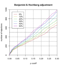
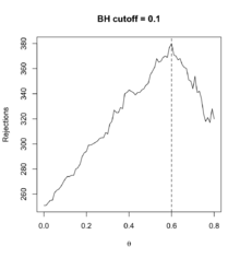
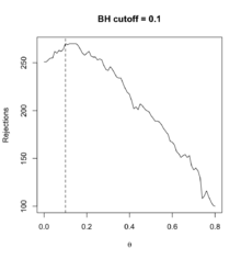
- DESeq2 Independent filtering of results. Independent filtering is performed AFTER the differential expression analysis (DEA) in DESeq2.
- The results function of the DESeq2 package performs independent filtering by default using the mean of normalized counts as a filter statistic.
- A threshold on the filter statistic is found which optimizes the number of adjusted p values lower than a significance level alpha.
- The adjusted p values for the genes which do not pass the filter threshold are set to NA.
- StatQuest: edgeR and DESeq2, part 2. Mitigate the multiple testing problem. code, written guide.
- A simulated data shows FDR is doing a great job limiting number of False Positives in the significant results, but it's not awesome keeping the True Positives.
- Each time we increase the number of bogus tests, we reduce the number of True Positive p-values < .05 that survive the FDR adjustment.
- A plot of True/False Positives vs Number of bogus tests. That means FDR is still having its limitation.
The independent filtering helps address this limitation. - edgeR recommends removing all genes except those with > 1 CPM in 2 or more samples. It compensates for differences in read depth between libraries. The CPM cutoff "1" depends on the data. How can we determine what a good CPM cutoff is?.
- Differences of edgeR and DESeq2.
- Y-axis is number of significant genes, X-axis is the threshold/quantiles. Choose the threshold/quantile such that the number of significant genes is maximized.
- Advice. We see the filtering was done after calculating p-values.
- Sensitivity, Specificity, ROC, Multiple testing, Independent filtering by Wolfgang Huber.
- Independent filtering increases detection power for high-throughput experiments. Richard Bourgon 2010.
- Exploring DESeq2 results: Wald test. 3. Genes with a low mean normalized counts.
- DESeq vs edgeR Comparison.


edgeR::filterByExpr
- ?filterByExpr
- limma user guide
- Is it okay to increase filtering to get more significant Adjusted P Values for DEGs found using Limma?
- DESeq2 filtering vs edgeR filtering
Normalization
- How data analysis affects power, reproducibility and biological insight of RNA-seq studies in complex datasets 2015
- Comparing the normalization methods for the differential analysis of Illumina high-throughput RNA-Seq data 2015
- Expression analysis of RNA sequencing data from human neural and glial cell lines depends on technical replication and normalization methods 2018
- A statistical normalization method and differential expression analysis for RNA-seq data between different species Zhou 2019
- RNA-seq analysis some notes from Ming Tang
- A protocol to evaluate RNA sequencing normalization methods Abrams et al 2019. It concluded that transcripts per million (TPM) was the best performing normalization method based on its preservation of biological signal as compared to the other methods tested.
- Data pre-processing 6.6.3 Normalising gene expression distributions. log2 CPM (counts per million) was considered. edgeR::calcNormFactors(x, method = "TMM") was used to normalize counts.
- Generalized Linear Models and Plots with edgeR – Advanced Differential Expression Analysis
- CrossNorm: a novel normalization strategy for microarray data in cancers Cheng 2016
- EnrichmentBrowser::normalize()
- SingleCellExperiment vignette. It lists 4 special assays: counts, logcounts, cpm and tpm.
- 8.3.4 Within sample normalization of the read counts and 8.3.5 Computing different normalization schemes in R from Computational Genomics with R by Altuna Akalin
- CPM is the simplest method. It addresses the sequencing depth bias by normalizing the read counts per gene by dividing each gene’s read count by a certain value and multiplying it by 10^6. There are 3 ways for the denominator: Total Counts Normalization, Upper Quartile Normalization and Median Normalization.
- Popular metrics that improve upon CPM are RPKM/FPKM (reads/fragments per kilobase of million reads) and TPM (transcripts per million).
- RPKM is obtained by dividing the CPM value by another factor, which is the length of the gene per kilobase. FPKM (substitute reads with fragments) is the same as RPKM, but is used for paired-end reads. So RPKM differs from CPM by adding one step.
- TPM also controls for both the library size and the gene lengths, however, with the TPM method, the read counts are first normalized by the gene length (per kilobase), and then gene-length normalized values are divided by the sum of the gene-length normalized values and multiplied by 10^6.
- Library composition or RNA composition. In DESeq2 the read counts are normalized by computing size factors, which addresses the differences not only in the library sizes, but also the library compositions. See 8.3.7 Differential expression analysis
- Different samples contain different active genes
- This procedure corrects for library size and RNA composition bias, which can arise for example when only a small number of genes are very highly expressed in one experiment condition but not in the other.
- DESeq2 first normalizes the count data to account for differences in library sizes and RNA composition between samples.
- A few highly differentially expressed genes between samples, differences in the number of genes expressed between samples, or presence of contamination can skew some types of normalization methods. Introduction to DGE gives a nice graphical illustration of RNA composition.
- StatQuest: DESeq2, part 1, Library Normalization - adjusting for differences in library composition
- Sequencing bias detection from RNA composition from the NOISeq's vignette.
- Selecting between-sample RNA-Seq normalization methods from the perspective of their assumptions Evans 2018. R code is in github. seqc package from Bioconductor.
- Evaluation of critical data processing steps for reliable prediction of gene co-expression from large collections of RNA-seq data Vandenbon 2021. Methods that correct for differences in gene length (RPKM and FPKM) don't affect correlation value; that is, these methods would be equivalent to CPM normalization.
- TPM, FPKM, or Normalized Counts? A Comparative Study of Quantification Measures for the Analysis of RNA-seq Data from the NCI Patient-Derived Models Repository Zhao 2021
- Youtube
- Robust normalization and transformation techniques for constructing gene coexpression networks from RNA-seq data 2022
log2 transformation
No matter we use TPM, TMM, FPKM, or DESeq2 normalized counts, we still need to take a log2(x+1) transformation before any analyses.
Quantile normalization
- https://en.wikipedia.org/wiki/Quantile_normalization. The new values are the averaged ordered values per gene based on the original rank.
- Mastering Quantile Normalization in R: A Step-by-Step Guide. The quantiles of the normalized data are consistent across the different datasets.
- Question: Quantile normalizing prior to or after TPM scaling?
- When to use Quantile Normalization? and its R package quantro
- Quantile normalisation in R
- normalize.quantiles() from preprocessCore package. How to Perform Quantile Normalization in R
- for ties, the average is used in normalize.quantiles(), ((4.666667 + 5.666667) / 2) = 5.166667.
- I got into an error when I use the function in RStudio docker container but the solution here (BiocManager::install("preprocessCore", configure.args="--disable-threading")) works.
source('http://bioconductor.org/biocLite.R')
biocLite('preprocessCore')
#load package
library(preprocessCore)

#the function expects a matrix
#create a matrix using the same example
mat <- matrix(c(5,2,3,4,4,1,4,2,3,4,6,8),
             ncol=3)
mat
#     [,1] [,2] [,3]
#[1,]    5    4    3
#[2,]    2    1    4
#[3,]    3    4    6
#[4,]    4    2    8

#quantile normalisation
normalize.quantiles(mat)
#         [,1]     [,2]     [,3]
#[1,] 5.666667 5.166667 2.000000
#[2,] 2.000000 2.000000 3.000000
#[3,] 3.000000 5.166667 4.666667
#[4,] 4.666667 3.000000 5.666667
Distribution, density plot
Density plot showing the distribution of RNA-seq read counts (FPKM) log10(FPKM)
Negative binomial distribution
RNA-seq and Negative binomial distribution
Z-score transformation
- This practice has been used extensively in papers without a clear foundation.
- Analysis of Microarray Data Using Z Score Transformation Cheadle 2003. Z-normalization was calculated per gene.
- For example, ssGSEA score-based Ras dependency indexes derived from gene expression data reveal potential Ras addiction mechanisms with possible clinica implications applies z-scores on each gene AND ssGSEA scores for each pathway/gene signature.
- Transforming RNA-Seq Data to Improve the Performance of Prognostic Gene Signatures Zwiener 2014. Often, standardizing gene expressions is implemented as a default in software packages.
- RNAseq: Z score, Intensity, and Resources. For visualization in heatmaps or for other clustering (e.g., k-means, fuzzy) it is useful to use z-scores.
Ensembl to gene symbol
- http://useast.ensembl.org/index.html (seems down). Training.
- Online tools
- R. Gene ID mapping using R.
- AnnotationDbi::mapIds() function + "org.Hs.eg.db" package. It works well.
- Vignette of EnhancedVolcano package
- Converting Gene Names in R with AnnotationDbi
- my TCGAbiolinks-GBM.Rmd.
- getBM() from "biomaRt" package
- ensembl_to_symbol() from tidybulk package.
- A Tidy Transcriptomics introduction to RNA sequencing analyses (Bioc 2020).
- AnnotationDbi::mapIds() function + "org.Hs.eg.db" package. It works well.
How to use UCSC Table Browser
- An instruction from BitSeq software
- How To Get Bed File Containing Exons Of Canonical Transcripts And Their Corresponding Gene Symbols
- Where to download refseq gene coding regions data?
- http://genome.ucsc.edu/cgi-bin/hgTables OR
- Download refGene.txt.gz file from UCSC directly using http links
- Where To Download Genome Annotation Including Exon, Intron, Utr, Intergenic Information?
File:Tablebrowser.png File:Tablebrowser2.png
Note
- the UCSC browser will return the output on browser by default. Users need to use the browser to save the file with self-chosen file name.
- the output does not have a header
- The bed format is explained in https://genome.ucsc.edu/FAQ/FAQformat.html#format1
If I select "Whole Genome", I will get a file with 75,893 rows. If I choose "Coding Exons", I will get a file with 577,387 rows.
$ wc -l hg38Tables.bed
75893 hg38Tables.bed
$ head -2 hg38Tables.bed
chr1	67092175	67134971	NM_001276352	0	-	67093579	67127240	0	9	1429,70,145,68,113,158,92,86,42,	0,4076,11062,19401,23176,33576,34990,38966,42754,
chr1	201283451	201332993	NM_000299	0	+	201283702	201328836	0	15	453,104,395,145,208,178,63,115,156,177,154,187,85,107,2920,	0,10490,29714,33101,34120,35166,36364,36815,38526,39561,40976,41489,42302,45310,46622,
$ tail -2 hg38Tables.bed
chr22_KI270734v1_random	131493	137393	NM_005675	0	+	131645	136994	0	5	262,161,101,141,549,	0,342,3949,4665,5351,
chr22_KI270734v1_random	138078	161852	NM_016335	0	-	138479	161586	0	15	589,89,99,176,147,93,82,80,117,65,150,35,209,313,164,	0,664,4115,5535,6670,6925,8561,9545,10037,10335,12271,12908,18210,23235,23610,

$ wc -l hg38CodingExon.bed
577387 hg38CodingExon.bed
$ head -2 hg38CodingExon.bed
chr1	67093579	67093604	NM_001276352_cds_0_0_chr1_67093580_r	0	-
chr1	67096251	67096321	NM_001276352_cds_1_0_chr1_67096252_r	0	-
$ tail -2 hg38CodingExon.bed
chr22_KI270734v1_random	156288	156497	NM_016335_cds_12_0_chr22_KI270734v1_random_156289_r	0	-
chr22_KI270734v1_random	161313	161586	NM_016335_cds_13_0_chr22_KI270734v1_random_161314_r	0	-

# Focus on one NCBI refseq (https://www.ncbi.nlm.nih.gov/nuccore/444741698)
$ grep NM_001276352 hg38Tables.bed
chr1	67092175	67134971	NM_001276352	0	-	67093579	67127240	0	9	1429,70,145,68,113,158,92,86,42,	0,4076,11062,19401,23176,33576,34990,38966,42754,
$ grep NM_001276352 hg38CodingExon.bed
chr1	67093579	67093604	NM_001276352_cds_0_0_chr1_67093580_r	0	-
chr1	67096251	67096321	NM_001276352_cds_1_0_chr1_67096252_r	0	-
chr1	67103237	67103382	NM_001276352_cds_2_0_chr1_67103238_r	0	-
chr1	67111576	67111644	NM_001276352_cds_3_0_chr1_67111577_r	0	-
chr1	67115351	67115464	NM_001276352_cds_4_0_chr1_67115352_r	0	-
chr1	67125751	67125909	NM_001276352_cds_5_0_chr1_67125752_r	0	-
chr1	67127165	67127240	NM_001276352_cds_6_0_chr1_67127166_r	0	-
This can be compared to refGene(?) directly downloaded via http
$ wget -c -O hg38.refGene.txt.gz http://hgdownload.soe.ucsc.edu/goldenPath/hg38/database/refGene.txt.gz
--2018-10-09 15:44:43--  http://hgdownload.soe.ucsc.edu/goldenPath/hg38/database/refGene.txt.gz
Resolving hgdownload.soe.ucsc.edu (hgdownload.soe.ucsc.edu)... 128.114.119.163
Connecting to hgdownload.soe.ucsc.edu (hgdownload.soe.ucsc.edu)|128.114.119.163|:80... connected.
HTTP request sent, awaiting response... 200 OK
Length: 7457957 (7.1M) [application/x-gzip]
Saving to: ‘hg38.refGene.txt.gz’

hg38.refGene.txt.gz                100%[===============================================================>]   7.11M   901KB/s    in 10s

2018-10-09 15:44:54 (708 KB/s) - ‘hg38.refGene.txt.gz’ saved [7457957/7457957]

$ zcat hg38.refGene.txt.gz | wc -l
75893
15:45PM /tmp$ zcat hg38.refGene.txt.gz | head -2
1072	NM_003288	chr20	+	63865227	63891545	63865365	63889945	7	63865227,63869295,63873667,63875815,63882718,63889189,63889849,	63865384,63869441,63873816,63875875,63882820,63889238,63891545,	0	TPD52L2	cmpl	cmpl	0,1,0,2,2,2,0,
1815	NR_110164	chr2	+	161244738	161249050	161249050	161249050	2	161244738,161246874,	161244895,161249050,	0	LINC01806	unk	unk	-1,-1,

$ zcat hg38.refGene.txt.gz | tail -2
1006	NM_130467	chrX	+	55220345	55224108	55220599	55224003	5	55220345,55221374,55221766,55222620,55223986,	55220651,55221463,55221875,55222746,55224108,	0	PAGE5	cmpl	cmpl	0,1,0,1,1,
637	NM_001364814	chrY	-	6865917	6874027	6866072	6872608	7	6865917,6868036,6868731,6868867,6870005,6872554,6873971,	6866078,6868462,6868776,6868909,6870053,6872620,6874027,	0	AMELY	cmpl	cmpl	0,0,0,0,0,0,-1,
Where to download reference genome
- UCSC and twoBitToFa to UCSC convert .2bit to fasta.
- hg19 from UCSC (chromosome-wise).
Which human reference genome to use?
http://lh3.github.io/2017/11/13/which-human-reference-genome-to-use (11/13/2017)
UHR, HBR
In RNA sequencing (RNA-seq), Universal Human Reference (UHR) and Human Brain Reference (HBR) are two types of commercially available RNA samples that are often used as control samples and assess the performance and accuracy of RNA-seq assays. See this (github) and Lesson 13: Aligning raw sequences to reference genome.
GENCODE transcript database
RefSeq categories
See Table 1 of Chapter 18The Reference Sequence (RefSeq) Database.
| Category | Description |
|---|---|
| NC | Complete genomic molecules |
| NG | Incomplete genomic region |
| NM | mRNA |
| NR | ncRNA |
| NP | Protein |
| XM | predicted mRNA model |
| XR | predicted ncRNA model |
| XP | predicted Protein model (eukaryotic sequences) |
| WP | predicted Protein model (prokaryotic sequences) |
UCSC version & NCBI release corresponding
Gene Annotation
- GeneCards
- Genetics Home Reference from National Library of Medicine
- My Cancer Genome
- Cosmic
- annotables R package.
- ensembldb R package
- https://www.gencodegenes.org/human/releases.html
- For gene symbols, there are NCBI and HUGO. See an example from GSE6532 (annot.tam object).
library(rtracklayer)
genes <- readGFF("gencode.v27.annotation.gff3.gz")
genes[1:2, 1:5]
# DataFrame with 2 rows and 5 columns
#      seqid   source       type     start       end
#   <factor> <factor>   <factor> <integer> <integer>
# 1     chr1   HAVANA gene           11869     14409
# 2     chr1   HAVANA transcript     11869     14409
genes[1:100, ] %>% filter(type == "gene") %>% dim()
# Error in UseMethod("filter") :
#   no applicable method for 'filter' applied to an object of class "c('DFrame', 'DataFrame', 'RectangularData', 'SimpleList', 'DataFrame_OR_NULL', 'List', 'Vector', 'list_OR_List', 'Annotated', 'vector_OR_Vector')"

library(ape)
genes2 <- read.gff("gencode.v27.annotation.gff3.gz")
genes2[1:2, 1:5]
#   seqid source       type start   end
# 1  chr1 HAVANA       gene 11869 14409
# 2  chr1 HAVANA transcript 11869 14409
genes2[1:100,]  %>% filter(type == "gene") %>% dim()
# [1] 11  9
Genecards
- https://www.genecards.org/
- Q: What are genes with gene symbols starting with LINC?; eg LINC00491
A: Genes with gene symbols starting with "LINC" are long intergenic non-coding RNA (lncRNA) genes. lncRNAs are RNA molecules that are transcribed from the genome but do not encode proteins. Unlike protein-coding genes, lncRNAs do not have a well-defined coding sequence, but they do play important regulatory roles in cellular processes such as gene expression, chromatin structure, and genome stability. Some lncRNAs are specifically expressed in cancer cells and have been implicated in tumor development and progression, making them of interest for cancer research.
How many DNA strands are there in humans?
- http://www.numberof.net/number-of-dna-strands/
- http://www.answers.com/Q/How_many_DNA_strands_are_there_in_humans
How many base pairs in human
- 3 billion base pairs. https://en.wikipedia.org/wiki/Human_genome
- chromosome 22 has the smallest number of bps (~50 million).
- chromosome 1 has the largest number of bps (245 million base pairs).
- Illumina iGenome Homo_sapiens/UCSC/hg19/Sequence/WholeGenomeFasta/genome.fa file is 3.0GB (so is other genome.fa from human).
Gene, Transcript, Coding/Non-coding exon
- https://hslnews.wordpress.com/2015/07/02/bioinformatics-bite-how-to-find-the-transcription-start-site-of-a-gene/
- According to https://en.wikipedia.org/wiki/Exon, in the human genome only
- 1.1% of the genome is spanned by exons,
- 24% is in introns,
- 75% of the genome being intergenic DNA.
- https://twitter.com/ensembl/status/1276469013707665410?s=20
SNP
Types of SNPs and number of SNPs in each chromosomes
NGS technology
DNA methylation, Epigenetics
- Relation of methylation genes and gene expression
- Methylation of genes can have different effects on gene expression, depending on where the methylation occurs in the gene and the specific context of the gene and the cellular environment. Generally, methylation of promoter regions of genes is associated with reduced gene expression, whereas methylation of gene body regions is less clearly associated with gene expression changes.
- When DNA is methylated at the promoter region of a gene, it can prevent the binding of transcription factors and RNA polymerase, which are necessary for transcription initiation. Methylation at the promoter region can also recruit proteins that block transcription or promote histone modifications that lead to chromatin compaction, further limiting access to the gene for transcriptional machinery.
- However, methylation in other regions of the gene, such as the gene body, can have more complex effects on gene expression. In some cases, gene body methylation can be associated with increased expression, while in other cases it may have no effect or even lead to decreased expression. It is thought that gene body methylation may be involved in regulating alternative splicing or RNA stability, among other possible mechanisms.
- Therefore, the effect of methylation on gene expression is not always straightforward and depends on various factors, including the specific gene, the location of methylation, and the cellular context.
- DNA Methylation - Biochemistry (USMLE Step 1)
- DNA methylation = InActivates DNA transcription
- The level of mRNA expression is inversely related to the extent of methylation. See this screenshot example from TCGA
- hemimethylated DNA vs allele-specific methylation. DNA-hemimethylation is when only one of two (complementary) strands is methylated.
- methylationArrayAnalysis : A cross-package Bioconductor workflow for analysing methylation array data
- Comparison of Beta-value and M-value methods for quantifying methylation levels by microarray analysis Du 2010. Figure 3 shows scatterplots of SD vs mean based on technical replicates of using beta or M-value. It can be seen M-value satisfies homoscedasticity but beta does not.
- Is Your DNA Your Destiny? A Primer on Epigenetics
- GC content = (G+C)/(A+T+G+C) x 100%
- How many CpGs (C follows by G)?
- Some papers
- Identification of prostate cancer specific methylation biomarkers from a multi-cancer analysis 2021. Within all bootstrapped datasets, sites with non-zero coefficients in more than 99% LASSO models were kept.
- Analyzing DNA methylation data (part of the book Biomedical Data Science) and the PH525x: Data Analysis for Genomics (edX course). The Github website is on https://github.com/genomicsclass/labs. The source code may not be correct. See also http://www.biostat.jhsph.edu/~iruczins/teaching/kogo/html/ml/week8/methylation.Rmd. The paper Bump hunting to identify differentially methylated regions in epigenetic epidemiology studies the tutorial has mentioned.
devtools::install_github("coloncancermeth","genomicsclass")
library(coloncancermeth) # 485512 x 26
data(coloncancermeth) # load meth (methylation data), pd (sample info ) and gr objects
dim(meth)
dim(pd)
length(gr)
colnames(pd)
table(pd$Status) # 9 normals, 17 cancers
normalIndex <- which(pd$Status=="normal")
cancerlIndex <- which(pd$Status=="cancer")

i=normalIndex[1]
plot(density(meth[,i],from=0,to=1),main="",ylim=c(0,3),type="n")
for(i in normalIndex){
  lines(density(meth[,i],from=0,to=1),col=1)
}
### Add the cancer samples
for(i in cancerlIndex){
  lines(density(meth[,i],from=0,to=1),col=2)
}

# finding regions of the genome that are different between cancer and normal samples
library(limma)
X<-model.matrix(~pd$Status)
fit<-lmFit(meth,X)
eb <- ebayes(fit)

# plot of the region surrounding the top hit
library(GenomicRanges)
i <- which.min(eb$p.value[,2])
middle <- gr[i,]
Index<-gr%over%(middle+10000)
cols=ifelse(pd$Status=="normal",1,2)
chr=as.factor(seqnames(gr))
pos=start(gr)

plot(pos[Index],fit$coef[Index,2],type="b",xlab="genomic location",ylab="difference")
matplot(pos[Index],meth[Index,],col=cols,xlab="genomic location")
# http://www.ncbi.nlm.nih.gov/pubmed/22422453

# within each chromosome we usually have big gaps creating subgroups of regions to be analyzed
chr1Index <- which(chr=="chr1")
hist(log10(diff(pos[chr1Index])),main="",xlab="log 10 method")

library(bumphunter)
cl=clusterMaker(chr,pos,maxGap=500)
table(table(cl)) ##shows the number of regions with 1,2,3, ... points in them
#consider two example regions#
...
Integrate DNA methylation and gene expression
- iNETgrate: Integrates DNA methylation data with gene expression in a single gene network. Paper 2023.
- ELMER Inferring Regulatory Element Landscapes and Transcription Factor Networks Using Cancer Methylomes and Paper 2019.
- Integrative analysis of DNA methylation and gene expression identified cervical cancer-specific diagnostic biomarkers 2019
- EnrichedHeatmap: an R/Bioconductor package for comprehensive visualization of genomic signal associations 2018
- TCGAbiolinks vignette. Case 3. Create a scatterplot of log10(FDR gene expression) vs log10(FDR dna methylation). Case 4. ELMER - Identify putative target genes for differentially methylated distal probes, using methylation vs. expression correlation. Identify master regulatory Transcription Factors (TF) whose expression associate with DNA methylation changes at multiple regulatory regions.
Whole Genome Sequencing, Whole Exome Sequencing, Transcriptome (RNA) Sequencing
- http://www.rna-seqblog.com/exome-sequencing-vs-rna-seq-to-identify-coding-region-variants/
- http://www.rna-seqblog.com/combined-use-of-exome-and-transcriptome-sequencing/
- A comparison of whole genome and whole transcriptome sequencing
Sequence + Expression
Integrate RNA-Seq and DNA-Seq
- Integrated RNA and DNA sequencing reveals early drivers of metastatic breast cancer by Perou. An R code is provided.
Immunohistochemistry/IHC
https://en.wikipedia.org/wiki/Immunohistochemistry. Protein expression by IHC.
Deconvolve bulk tumor tissue
Performance of computational algorithms to deconvolve heterogeneous bulk tumor tissue depends on experimental factors. Twitter.
Tumor purity
- Tumor Purity in Preclinical Mouse Tumor Models 2022
- Systematic Assessment of Tumor Purity and Its Clinical Implications Haider 2020.
- With the exception of naive miRNA profiles, purity estimates were inversely correlated with molecular profiles regardless of the underlying purity estimation profile .
- These data suggest that the presence of genomic and transcriptomic correlates of tumor purity are likely to confound biologic and clinical interpretations.
- Estimators:
- DNA: ABSOLUTE, ASCAT, CLONET, INTEGER, OncoSNP
- RNA: DeMix, ISOpure-R (matlab/R), ESTIMATE (Yoshihara, R)
- miRNA/microRNA: ISOpure-I
- TCGA purity estimate by Aran 2015 Systematic pan-cancer analysis of tumour purity - Supplementary Data 1 (xlsx file with columns: Sample ID,Cancer type,ESTIMATE,ABSOLUTE,LUMP,IHC & CPE).
- Tumor.purity: TCGA samples with their Tumor Purity measures (a data frame with 9364 rows and 7 variables) from TCGAbiolinks package
- Prediction of tumor purity from gene expression data using machine learning 2021.
- We selected the CPE as the target variable, which is the median purity value after normalizing values from the other four purity estimates (ESTIMATE, ABSOLUTE, LUMP and IHC).
- our data set consisted of 8405 tumor samples.
- How VAF is related to tumor purity?
- Variant allelic fraction (VAF) is related to tumor purity because it reflects the proportion of cells in a sample that carry a specific genetic variant. In the context of cancer, VAF can be used as a surrogate marker for tumor purity, as the fraction of cells in the sample that carry the variant will depend on the proportion of cancer cells relative to normal cells.
- The VAF of a specific genetic variant in a cancer sample can be calculated as the ratio of the number of reads supporting the variant to the total number of reads covering that locus. In a sample that is purely composed of cancer cells, the VAF should approach 1, as all cells will carry the variant. In a sample that is mixed with normal cells, the VAF will be lower and proportional to the proportion of cancer cells in the sample.
- Therefore, by measuring the VAF of one or more genetic variants, it is possible to estimate the tumor purity, which is the proportion of cancer cells in the sample relative to normal cells. This information is important for a variety of downstream analyses, including variant calling, gene expression analysis, and the estimation of the mutational burden, as it can affect the interpretation of the results and the accuracy of the analysis.
- How gene expression can be used to estimate tumor purity?
- Gene expression analysis can be used to estimate tumor purity by comparing the expression levels of genes known to be specific to either normal or cancer cells. In a sample that is mixed with normal and cancer cells, the expression levels of these genes will reflect the proportion of normal and cancer cells present in the sample.
- For example, genes that are highly expressed in normal cells, such as housekeeping genes, can be used as a reference to estimate the proportion of normal cells in the sample. Similarly, genes that are highly expressed in cancer cells, such as oncogenes, can be used to estimate the proportion of cancer cells in the sample.
- The relative expression levels of these genes can then be used to estimate the tumor purity, either by comparing the expression levels to a reference sample of known purity, or by using mathematical models to estimate the proportion of normal and cancer cells in the sample.
- It is important to note that this method is not without limitations, as the expression levels of specific genes can be influenced by various factors, such as the presence of cell-to-cell heterogeneity, gene amplification, and epigenetic modifications, among others. Therefore, gene expression analysis should be used in combination with other methods, such as copy number analysis and variant allelic fraction analysis, to obtain a more accurate estimate of tumor purity.
- Some papers
- Tumor purity as a prognosis and immunotherapy relevant feature in gastric cancer
- Identifying driver mutations in sequenced cancer genomes: computational approaches to enable precision medicine. Tumor purity affects the detection of somatic mutations. Explain in plot about what are heterozygous somatic SNV and one hetererozygous germline SNV.
- ISOpureR (Quon 2013): intensity or count data. Error term [math]\displaystyle{ e_n }[/math] multinomial distribution.
library(ISOpureR)

# For reproducible results, set the random seed
set.seed(123);

# Run ISOpureR Step 1 - Cancer Profile Estimation
system.time(ISOpureS1model <- ISOpure.step1.CPE(
  tumor.expression.data,  # intensity or count data
  normal.expression.data  # intensity or count data
))
ISOpureS1model$alphapurities  # tumor purity estimates
- ESTIMATE (Yoshihara 2013): normalized data.
- Since it is based ssGSEA, only ranks are used. It does not matter we used the log transformed or count data.
- ssGSEA is based on two gene signatures: Stromal signature (141 genes) and immune signature (141 genes)
- The formula for calculating ESTIMATE tumor purity was developed in TCGA Affymetrix data (n=1001) including both the ESTIMATE score and ABSOLUTE-based tumor purity.
- An evolutionary algorithm was used for the mathematical model.
- Nonlinear least squares method was used to determine the final model estimate.
- Tumor purity = cos(0.6 + 0.000146 * ESTIMATE score)
library(estimate) OvarianCancerExpr <- system.file("extdata", "sample_input.txt", package="estimate") filterCommonGenes(input.f=OvarianCancerExpr, output.f="OV_10412genes.gct", id="GeneSymbol") estimateScore("OV_10412genes.gct", "OV_estimate_score.gct", platform="affymetrix") plotPurity(scores="OV_estimate_score.gct", samples="s516", platform="affymetrix") scan("OV_estimate_score.gct", "", skip=6)[-c(1:2)] |> as.numeric() # tumor purity estimates - DeMixT (Wang 2018): count data. Estimation of tumor cell total mRNA expression in 15 cancer types predicts disease progression, Cao 2022 for profile likelihood method & supplementary information for more information about the benchmarking between DeMixT_DE and DeMixT_GS.
library(DeMixT) source("DeMixT_preprocessing.R") count.mat <- cbind(normal.expression.data, tumor.expression.data) colnames(count.mat) <- paste0("sample", 1:ncol(count.mat)) label = factor(c(rep('Normal', ncol(normal.expression.data)), rep('Tumor', ncol(tumor.expression.data)))) set.seed(1234) # not sure if this is needed preprocessed_data = DeMixT_preprocessing(count.mat, label) PRAD_filter = preprocessed_data$count.matrix set.seed(1234) Normal.id <- paste0("sample", 1:n1) Tumor.id <- paste0("sample", (n1+1):(n1+n2)) data.Y = SummarizedExperiment(assays = list(counts = PRAD_filter[, Tumor.id])) data.N1 <- SummarizedExperiment(assays = list(counts = PRAD_filter[, Normal.id])) res = DeMixT(data.Y = data.Y, data.N1 = data.N1, nthread = 64, gene.selection.method = "DE") # default is "GS" res$pi[2, ] # tumor purity estimates - CIBERSORTx (Newman 2019). Web only. Determining cell type abundance and expression from bulk tissues with digital cytometry
- PUREE (Revkov 2023). Python-based. Only API, no source code.
Integrate/combine Omics
- awesome-multi-omics by Michael Love
- Ten quick tips for avoiding pitfalls in multi-omics data integration analyses 2023
- BloodCancerMultiOmics2017. "Drug-perturbation-based stratification of blood cancer" by Dietrich S, Oles M, Lu J et al. - experimental data and complete analysis.
- OmicsPLS & the paper in BMC Bioinformatics 2018
- MultiAssayExperiment & the paper in AACR 2017
- mixOmics, http://mixomics.org/, the paper on PLOS 2017
- The impact of different sources of heterogeneity on loss of accuracy from genomic prediction models Biostatistics 2018
- Tweedieverse, Github
- Combining gene mutation with gene expression data improves outcome prediction in myelodysplastic syndromes 2015, R code for Supplementary Data 2 and 4 and mg14.R.
- A comprehensive database for integrated analysis of omics data in autoimmune diseases 2021
- Integrative survival analysis of breast cancer with gene expression and DNA methylation data Bichindaritz, 2021
- Machine learning to analyse omic-data for COVID-19 diagnosis and prognosis 2023
Gene expression
Expression level is the amount of RNA in cell that was transcribed from that gene. Slides from Alyssa Frazee.
Fusion gene
- https://en.wikipedia.org/wiki/Fusion_gene
- https://github.com/STAR-Fusion/STAR-Fusion,
- Gene fusion discovery
- chimeraviz Visualization tools for gene fusions
- Tools to call fusions & Common issues with fusion calling, visualizing fusion events in IGV
Structural variation
- https://en.wikipedia.org/wiki/Structural_variation
- https://www.ncbi.nlm.nih.gov/dbvar/content/overview/
- Detection of complex structural variation from paired-end sequencing data Joseph G. Arthur, 2018
LUMPY, DELLY, ForestSV, Pindel, breakdancer , SVDetect.
Covid-19
Bulk RNA sequencing for analysis of post COVID-19 condition 2024. 13 differentially expressed genes associated with PCC (long Covid) were found. Enriched pathways were related to interferon-signalling and anti-viral immune processes.
RNASeq + ChipSeq
Labs
Biowulf2 at NIH
- Main site: http://hpc.nih.gov
- User guide: https://hpc.nih.gov/docs/user_guides.html
- Unlock account (60 days inactive) https://hpc.nih.gov/dashboard/
- Transitioning from PBS to Slurm: https://hpc.nih.gov/docs/pbs2slurm.html
- Job Submission 'cheat sheet': https://hpc.nih.gov/docs/biowulf2-handout.pdf
- STAR: https://hpc.nih.gov/apps/STAR.html
BamHash
Hash BAM and FASTQ files to verify data integrity. The C++ code is based on OpenSSL and seqan libraries.
Reproducibility
- Improving reproducibility in computational biology research
- SnakeChunks: modular blocks to build Snakemake workflows for reproducible NGS analyses by Claire Rioualen et al, 2017.
Selected Papers
- Testing for association between RNA-Seq and high-dimensional data and the Bioconductor package globalSeq.
- The FDA’s Experience with Emerging Genomics Technologies—Past, Present, and Future
- Differential analysis of gene regulation at transcript resolution with RNA-seq Trapnell et al, Nature Biotechnology 31, 46–53 (2013)
- A Study of TP53 RNA Splicing Illustrates Pitfalls of RNA-seq Methodology
- Top RNA-Seq Articles – 2016 from RNA-Seq blog
- Multivariate association analysis with somatic mutation data by He 2017 Biometrics.
- RASflow – An RNA-Seq Analysis Workflow with Snakemake Zhang 2019
- A Survey of Bioinformatics Database and Software Usage through Mining the Literature
- Computational analysis of cancer genome sequencing data Cortés-Ciriano 2021. Focus on point mutations, copy number alterations, structural variations. For RNA-seq data, it focused on gene fusion detection.
Pictures
https://www.flickr.com/photos/genomegov
FISH/Fluorescence In Situ Hybridization
- [https://www.genome.gov/genetics-glossary/Fluorescence-In-Situ-Hybridization
- Fluorescent In Situ Hybridization (FISH) Assay
用DNA做身分鑑識
如何自学入门生物信息学
CRISPR
Staying current
Staying Current in Bioinformatics & Genomics: 2017 Edition
Papers
Common issues in algorithmic bioinformatics papers
What are some common issues I find when reviewing algorithmic bioinformatics conference papers?
Precision Medicine courses
Personalized medicine
- F.D.A. Approves First Gene-Altering Leukemia Treatment
- The FDA Just Approved a New Way of Fighting (lymphoma) Cancer Using Personalized Gene Therapy
- What is the difference between precision medicine and personalized medicine? What about pharmacogenomics? "personalized medicine" is an older term. Help Me Understand Genetics
- Predictive Biomarkers: Progress on the Road to Personalized Cancer Immunotherapy Emens 2021
Cancer and gene markers
- Colorectal cancer patients without KRAS mutations have far better outcomes with EGFR treatment than those with KRAS mutations.
- Two EGFR inhibitors, cetuximab and panitumumab are not recommended for the treatment of colorectal cancer in patients with KRAS mutations in codon 12 and 13.
- Breast cancer.
The shocking truth about space travel
bioSyntax: syntax highlighting for computational biology
https://bmcbioinformatics.biomedcentral.com/articles/10.1186/s12859-018-2315-y
Deep learning
Deep learning: new computational modelling techniques for genomics
HRD/homologous recombination deficiency 同源重组修复缺陷
- https://en.wikipedia.org/wiki/Homologous_recombination
- Homologous recombination proficient (HRP) cancer cells can repair DNA damage caused by chemotherapy, making them difficult to treat.
- drugs have been developed to target homologous recombination via c-Abl inhibition and to exploit (take advantage of) deficiencies in homologous recombination in cancer cells with BRCA mutations.
- One such drug is Olaparib, a PARP1 inhibitor that targets cancer cells by inhibiting base-excision repair (BER) in HR-deficient cells. However, cancer cells can become resistant to PARP1 inhibitors if they undergo deletions of mutations in BRCA2, restoring their ability to repair DNA by HR.
- https://www.genome.gov/genetics-glossary/homologous-recombination (graphical illustration). Homologous recombination is a type of genetic recombination in which nucleotide sequences are exchanged between two similar or identical molecules of DNA.
- BRCA1 and BRCA2 are genes that produce proteins responsible for repairing damaged DNA within cells. Mutations in these genes can lead to errors in the DNA repair process, resulting in an accumulation of mutations that can cause cancer. This condition is known as Homologous Recombination Deficiency (HRD). PARP inhibitors are a type of targeted therapy that blocks the enzyme Poly (ADP-ribose) polymerase (PARP), which helps repair DNA damage in (cancer) cells. By inhibiting PARP, these drugs prevent cancer cells from repairing their DNA, leading to cell death.
- The inability to repair DNA damage is referred to as homologous recombination deficiency (HRD). DNA damage response from Qiagen.
- openai
- Poly(ADP-ribose) polymerase (PARP) inhibitors are a class of drugs that are designed to inhibit the activity of PARP enzymes. PARP enzymes are proteins that are involved in DNA repair pathways. They help to repair DNA damage and maintain the stability of the genome by adding a chemical group called poly(ADP-ribose) to other proteins.
- PARP inhibitors work by blocking the activity of PARP enzymes, which can interfere with the ability of cells to repair damaged DNA. This can be especially useful in cancer cells, which often rely on PARP enzymes to repair DNA damage and maintain genomic stability. By inhibiting PARP enzymes, PARP inhibitors can sensitizize cancer cells to chemotherapy and other treatments, making them more vulnerable to cell death.
- is there drug targeting HRP cancer patients? One approach is to target homologous recombination via c-Abl inhibition. For example, Niraparib is a PARP inhibitor that has been shown to be effective in treating advanced ovarian cancer in both homologous recombination deficient (HRD) and homologous recombination proficient (HRP) patients.
- is there any drugs target HRD cancer patients? Yes, there are several drugs that have been developed to target HRD cancer cells. One approach is to use PARP inhibitors, which exploit deficiencies in homologous recombination in cancer cells with BRCA mutations. For example, Olaparib is a PARP1 inhibitor that has been shown to be effective in shrinking or stopping the growth of tumors from breast, ovarian and prostate cancers caused by mutations in the BRCA1 or BRCA2 genes. By inhibiting base-excision repair (BER) in HR-deficient cells, Olaparib applies the concept of synthetic lethality to specifically target cancer cells. PS: Examples of PARP inhibitors include niraparib (Zejula), olaparib (Lynparza), talazoparib (Talzenna), and rucaparib (Rubraca).
- PARP1 is a member of the PARP family of proteins. PARP stands for Poly (ADP-ribose) polymerase. The PARP family comprises 17 members.
- Loss-of-function genes involved in this pathway can sensitize tumors to poly(adenosine diphosphate [ADP]-ribose) polymerase (PARP) inhibitors and platinum-based (Pt) chemotherapy
- Certain genes that are involved in a process called Homologous Recombination Repair (HRR) can make cancer cells more susceptible to certain treatments. Specifically, it says that when these loss-of-function genes are present, the cancer cells become more sensitive to two types of chemotherapy: PARP inhibitors and platinum-based chemotherapy.
- Loss-of-function genes are genes that have mutations that prevent them from functioning properly or at all. By disrupting the normal functioning of the HRR pathway, these loss-of-function genes can make cancer cells more sensitive to PARP inhibitors and platinum-based chemotherapy.
- scarHRD package. Note for the 2 test samples, the return object is a 1x4 matrix.
- HRD-LOH/Loss of Heterozygosity
- LST/Large Scale Transitions
- Number of Telomeric Allelic Imbalances
- HRD-sum (sum of the above 3)
- Homologous Recombination Deficiency: Concepts, Definitions, and Assays Stewart 2022
- 同源重组修复缺陷HRD 分析
- 这篇只有两个Figure的10分+SCI是靠什么取胜的?
- HRD检测方法
- Link to HRD score, genome-wide DNA damage footprint. The HRD value has a range 0 to 101. Most are 0 and the rest follows an exponential distribution.
- Dynamically Accumulating Homologous Recombination Deficiency Score Served as an Important Prognosis Factor in High-Grade Serous Ovarian Cancer Su 2021
- A combined HRD score ≥42 was associated with shorter OS in 33 cancer types.
- However, in ovarian cancer, which ranked the highest HRD score among other cancers, HRD ≥42 cohort was significantly associated with longer OS.
- An HRD score of ≥42 was determined to signify HRD (HR-deficient), and a score of <42 was considered HR-proficient in clinical trials.
- The datasets including 1. signatures–HRD score and genome-wide DNA damage footprint; 2. phenotype-curated clinical data; and 3. gene expression RNAseq-TOIL RSEM TPM were downloaded from https://xenabrowser.net/.
- Identification of molecular subtypes and prognostic signature for hepatocellular carcinoma based on genes associated with homologous recombination deficiency Lin 2021.
- the combat function of R software package SVA was used for batch effect removal.
- https://xenabrowser.net/datapages/ has one set called "TCGA Pan-Cancer (PANCAN) (41 datasets)" -> HRD score, genome-wide DNA damage footprint (n=10,647) Pan-Cancer Atlas Hub.
- https://github.com/GerkeLab/TCGAhrd where HDR can be downloaded from https://gdc.cancer.gov/about-data/publications/PanCan-DDR-2018. Choose 'Zip file with TSV files of DDR Data Resources'. Pay attention to "DDRscores.tsv" and "Scores.tsv", "Samples.tsv".
- Homologous recombination deficiency in TCGA PanCancer Atlas
> load("clinical_and_hrd.RData") > dim(full_dat) [1] 9105 792 > full_dat[1:5, c("HRD_Score", "HRD_LOH", "HRD_LST", "HRD_TAI")] HRD_Score HRD_LOH HRD_LST HRD_TAI 1 7 2 2 3 2 9 3 2 4 3 0 0 0 0 4 8 4 2 2 5 5 1 1 3 > summary( full_dat[1:5, c("HRD_Score", "HRD_LOH", "HRD_LST", "HRD_TAI")]) HRD_Score HRD_LOH HRD_LST HRD_TAI Min. :0.0 Min. :0 Min. :0.0 Min. :0.0 1st Qu.:5.0 1st Qu.:1 1st Qu.:1.0 1st Qu.:2.0 Median :7.0 Median :2 Median :2.0 Median :3.0 Mean :5.8 Mean :2 Mean :1.4 Mean :2.4 3rd Qu.:8.0 3rd Qu.:3 3rd Qu.:2.0 3rd Qu.:3.0 Max. :9.0 Max. :4 Max. :2.0 Max. :4.0 > load("DDRscores.RData") > ls() [1] "dat" "full_dat" > dim(dat) [1] 9125 46 > colnames(dat) [1] "patient_id" "acronym" "mutLoad_silent" [4] "mutLoad_nonsilent" "mutSig1" "mutSig2" [7] "mutSig3" "mutSig4" "mutSig5" [10] "mutSig6" "mutSig7" "mutSig8" [13] "mutSig9" "mutSig10" "mutSig11" [16] "mutSig12" "mutSig13" "mutSig14" [19] "mutSig15" "mutSig16" "mutSig17" [22] "mutSig18" "mutSig19" "mutSig20" [25] "mutSig21" "CNA_n_segs" "CNA_frac_altered" [28] "CNA_n_focal_amp_del" "aneuploidy_score" "aneuploidy_score_prime" [31] "LOH_n_seg" "LOH_frac_altered" "purity" [34] "ploidy" "genome_doublings" "subclonal_frac" [37] "HRD_TAI" "HRD_LST" "HRD_LOH" [40] "HRD_Score" "eCARD" "PARPi7" [43] "PARPi7_bin" "RPS" "tp53_score" [46] "rppa_ddr_score" - HRD status is highly correlated with platinum chemotherapy sensitivity in patients with high-grade serous ovarian cancer (HGSOC) 2022. Findings showed that the HRD score of platinum treatment-sensitive patients was slightly higher than that of Pt-resistant patients. Analysis showed that patients with positive HRD status had a significantly longer progression-free survival (PFS) compared to those with negative HRD status.
- Effect of BRCA mutational status on survival outcome in advanced-stage high-grade serous ovarian cancer 2019. The median PFS was 22.9 months for the BRCA mutation group compared to 16.9 months for the wild-type BRCA group. 6 months was used as a cutoff.
- Ovarian Cancer Prognosis May Depend on Gene Mutations. Five-year survival rates were 61 percent for those with the BRCA2 mutation, 46 percent for those with the BRCA1 mutation and 36 percent for those with neither mutation, the investigators found.
- Homologous recombination deficiency status predicts response to platinum-based chemotherapy in Chinese patients with high-grade serous ovarian carcinoma 2023.
- HRD effects on first-line adjuvant chemotherapy and PARPi maintenance therapy in Chinese ovarian cancer patients 2023
- Pan-cancer landscape of homologous recombination deficiency 2020
- What to know about HRD testing for ovarian cancer
- HRD in Ovarian Cancer
- SAP for from Clovis Oncology & Rucaparib (a PARP inhibitor)
- gLOH vs LOH: The gLOH score and the LOH score are two different measures of Homologous Recombination Deficiency (HRD) in tumors. The gLOH score measures genomic loss of heterozygosity (gLOH) while the LOH score measures loss of heterozygosity (LOH) in a specific region or gene.
- What to know about HRD testing for ovarian cancer
- Labs:
- ACTHRD from ACT Genomics 行動基因. ACTHRD™ detects HRD status by LOH score and 24 HRR-related genes to evaluate whether a tumor is suitable for PARP inhibitors.
- AmoyDx. In-house testing for homologous recombination repair deficiency (HRD) testing in ovarian carcinoma: a feasibility study comparing AmoyDx HRD Focus panel with Myriad myChoiceCDx assay
- Bionano
- Burning Rock宣佈在中國獲得MyChoice®腫瘤檢測的許可
- FoundationMedicine (?FMI) technical information. Positive homologous recombination deficiency (HRD) status (F1CDx HRD defined as tBRCA-positive and/or LOH high) in ovarian cancer patients is associated with improved progression-free survival (PFS) from Rubraca (rucaparib) maintenance therapy in accordance with the Rubraca product label. FDA doc. Clinical and analytical validation of FoundationOne®CDx, a comprehensive genomic profiling assay for solid tumors 2022.
- Illumina
- Myriad
- Pillar Biosciences
- Sophia Genetics
- Tempus AI-DRIVEN HRD TEST
- Thermo fisher scientific Everything you need to know about homologous recombination repair (HRR) and homologous recombination deficiency (HRD) testing
Computational Pathology
- Computational pathology definitions, best practices, and recommendations for regulatory guidance: a white paper from the Digital Pathology Association 2019
- Challenges in Computational Pathology of Biomarker-Driven Predictive and Prognostic Immunotherapy
Bi-allelic, monoallelic
Bi-allelic and monoallelic expression. In most cases, both alleles (the two chromosomal copies) are transcribed; this is known as bi-allelic expression (left). However, a minority of genes show monoallelic expression (right). In these cases, only one allele of a gene is expressed (right).
SOMAscan assay (proteomic)
- https://somalogic.com/somascan-discovery/, https://somalogic.com/somascan-platform/, https://somalogic.com/user-manuals/
- SomaScan Assay v4.1 7k
- SomaDataIO R package (currently 6.0.0), Documentation including Vignettes.
f <- "SS-1234567_v4.1_Serum.hybNorm.medNormInt.plateScale.calibration.anmlQC.qcCheck.anmlSMP.adat"
my_adat <- read_adat(f)
eset <- adat2eSet(my_adat)

exprs(eset) |> dim() # 7596 x ns

pData(phenoData(eset)) # ns x 33
table(pData(phenoData(eset))$SampleType)

pData(featureData(eset)) # 7596 x 19
j2 <- pData(featureData(eset))$Organism == "Human" &
     (pData(featureData(eset))$Type %in% c("Protein", "Non-Human"))
sum(j2) # 7289
- SomaScan.db R package. v4.0 is 5K.
- SomaScan 11K Assay v5.0
- readat: An R package for reading and working with SomaLogic ADAT files
- https://bitbucket.org/graumannlabtools/readat/src/master/. The R package is not in Bioconductor.
- ToolViz package.
- NCBI-GEO, All list
- Assessment of variability in the plasma 7k SomaScan proteomics assay 2022
Scandal
阿茲海默症關鍵論文被揭發疑似造假,16年來全球醫學專家可能都被呼弄 & 阿茲海默症關鍵論文疑造假 誤導外界16年
Terms
RNA vs DNA
- Why RNA is a better measure of a patient’s current health than DNA
- 英美接種疫苗,陰謀論隨之盛行. 核糖核酸=RNA. 脱氧核糖核酸=DNA. 輝瑞公司開發的新冠疫苗,是使用mRNA疫苗原理,即抽取病毒內部分核糖核酸編碼蛋白(或者稱信使核糖核酸)制成疫苗。
- How mRNA Vaccines Work
- How Pfizer's RNA Vaccine Works
- Pfizer’s Covid Vaccine: 11 Things You Need to Know
- COVID-19 vaccine “95% effective”: It doesn’t mean what you think it means!
- Vaccine Technology: How MRNA Changed the Fight Against Covid-19
基因结构
https://zhuanlan.zhihu.com/p/49601643
Pseudogene
https://www.genome.gov/genetics-glossary/Pseudogene. An example: OR7E47P with alias bpl 41-16 or bpl41-16.
PCR
什麼是PCR? 聚合酶鏈鎖反應? 基因叔叔
Epidemiology
Epidemiology for the uninitiated
Cell lines
- cell line (體外). tumor samples (體內)
- A resource for cell line authentication, annotation and quality control
- Cell Lines: Types, Nomenclature, Selection and Maintenance (With Statistics)
- Comprehensive comparison of molecular portraits between cell lines and tumors in breast cancer Jiang 2016
- Evaluating cell lines as tumour models by comparison of genomic profiles Domcke 2013
- Google: tumor cell line vs tumor samples
in vivo, in vitro, and in situ
In silico 電腦模擬 (in silicon, s=simulation)
- https://en.wikipedia.org/wiki/In_silico An in silico experiment is one performed on computer or via computer simulation.
- The main difference between in silico gene expression analysis and experimental gene expression analysis is the method used to study the patterns and levels of gene expression.
- In silico gene expression analysis involves the use of computational tools and algorithms to analyze large datasets of gene expression data obtained from techniques such as microarrays, RNA sequencing, or single-cell RNA sequencing. This analysis can include identifying differentially expressed genes between samples, clustering genes with similar expression patterns, and predicting the functional roles of genes based on their expression profiles.
- On the other hand, experimental gene expression analysis involves directly measuring the levels and patterns of gene expression using laboratory techniques. These techniques can include real-time polymerase chain reaction (PCR), northern blotting, western blotting, and immunohistochemistry, among others. These experimental techniques allow researchers to directly measure the levels of specific RNA or protein molecules in biological samples.
- While in silico gene expression analysis is a rapid and cost-effective way to analyze large datasets of gene expression data, it relies on the accuracy and completeness of the data being analyzed. Experimental gene expression analysis provides a more direct and accurate view of gene expression but can be more time-consuming and expensive. In practice, both in silico and experimental gene expression analysis are valuable tools that can be used to complement each other in the study of gene expression and its role in various biological processes and diseases.
- In silico gene expression analysis--an overview Murray 2007
- A simple in silico approach to generate gene-expression profiles from subsets of cancer genomics data 2019
- TCGA from cbioportal was used
- Details steps including screenshots are available at Supplementary material
In situ 原處 (介於in vivo與in vitro之間)
- https://en.wikipedia.org/wiki/In_situ 意義大致介於in vivo與in vitro之間。
- Something that’s performed in situ means that it’s observed in its natural context, but outside of a living organism. In vivo is Latin for “within the living.” It refers to work that’s performed in a whole, living organism .
- A good example of this is a technique called in situ hybridization (ISH). ISH can be used to look for a specific nucleic acid (DNA or RNA) within something like a tissue sample. Specialized probes are used to bind to a specific nucleic acid sequence that the researcher is looking to find. These probes are tagged with things like radioactivity or fluorescence. This allows the researcher to see where the nucleic acid is located within the tissue sample. ISH allows the researcher to observe where a nucleic acid is located within its natural context, yet outside of a living organism. Examples are microarray experiments.
in vivo 活体内
- IN VIVO describes a medical experiment or a test that is performed on a living organism, e.g. a human being or a laboratory animal.
- Human primary cells and immortal cell lines: differences and advantages
- What is the Difference Between Primary Cell Culture and Cell Line
Syngenic
Syngeneic tumor models are experimental models used in cancer research that use genetically identical animals to study the growth and spread of cancer cells. In these models, a malignant tumor is induced in one animal and then transplanted into another animal of the same genetic background. This allows researchers to study the interactions between the host immune system and the cancer cells, as well as the response of the tumor to various treatments.
Syngeneic tumor models are often used in combination with other experimental models, such as xenograft models (where the cancer cells are transplanted into a genetically different animal) or cell line models (where the cancer cells are grown in a laboratory). By using a combination of these models, researchers can gain a more complete understanding of the biology of cancer and develop new treatments for cancer patients.
The syngeneic model is an important tool for studying the role of the immune system in cancer, as the genetically identical animals allow researchers to control for genetic differences that might impact the immune response. Additionally, because the host immune system in these models is functional and can mount a response against the transplanted cancer cells, the syngeneic model provides a more realistic representation of the host-tumor interaction than other models that rely on immunodeficient animals.
in vitro 试管内/体外
- https://en.wikipedia.org/wiki/In_vitro
- https://en.wikipedia.org/wiki/In_silico
- https://en.wikipedia.org/wiki/RNA-Seq
RUO: research use only
RUO stands for "Research Use Only". In the context of clinical trials and laboratory research, it refers to in vitro diagnostic products (IVDs) that are intended to be used in non-clinical studies, including to gather data for submission as required by regulatory authorities³. These products are not intended for use in diagnostic procedures. They are often used by medical laboratories and other institutions for research purposes. However, if these products are used for purposes other than research, it could have legal implications. It's important to note that RUO products are not subject to the same regulatory controls as in-vitro diagnostic medical devices (CE-IVDs) that must comply with the applicable legal requirements.
- Distribution of In Vitro Diagnostic Products Labeled for Research Use Only or Investigational Use Only
- In Vitro Diagnostic Use (IVD) versus Research Use Only (RUO) in the Clinical Laboratory
RNA sequencing 101
Web
- Introduction to Biology - The Secret of Life from edX. It's one of the top 100 best free online courses posted by ClassCentral.
- Introduction to RNA-Seq including biology overview (DNA, Alternative splcing, mRNA structure, human genome) and sequencing technology.
- Introduction to RNA-Seq for Researchers (youtube)
- RNA Sequencing 101 by Agilent Technologies. Includes the definition of sequencing depth (number of reads per sample) and coverage (number of reads/locus).
- What is a good sequencing depth for bulk RNA-Seq? In general 5 M mapped reads is a good bare minimum for a differential gene expression (DGE) analysis in human. In many cases 5 M – 15 M mapped reads are sufficient. Many published human RNA-Seq experiments have been sequenced with a sequencing depth between 20 M - 50 M reads per sample.
- How to count fastq reads echo $(zcat yourfile.fastq.gz | wc -l)/4 | bc
- Where do we get reads(A,C,T,G) from sample RNA? See page 12 of this pdf from Colin Dewey in U. Wisc.
- Quantification of RNA-Seq data (see the above pdf)
- Convert read counts into expression: RPKM (see the above pdf)
- RPKM and FPKM (Data analysis of RNA-seq from new generation sequencing by 張庭毓) RNA-Seq資料分析研討會與實作課程 / RNA Seq定序 / 次世代定序(NGS) / 高通量基因定序 分析.
- First vs Second generation sequence.
- The Simple Fool’s Guide to Population Genomics via RNASeq: An Introduction to HighThroughput Sequencing Data Analysis. This covers QC, De novo assembly, BLAST, mapping reads to reference sequences, gene expression analysis and variant (SNP) detection.
- An Introduction to Bioinformatics Resources and their Practical Applications from NIH library Bioinformatics Support Program.
- Teaching material from rnaseqforthenextgeneration.org which includes Designing RNA-Seq experiments, Processing RNA-Seq data, and Downstream analyses with RNA-Seq data.
Books
- RNA-seq Data Analysis: A Practical Approach. The pdf version is available on slideshare.net.
- Statistical Analysis of Next Generation Sequencing Data
- Modern Statistics for Modern Biology (free, see Statistics books) by Holmes and Huber. Plots are based on ggplot2.
- Learning Bioinformatics At Home - some resources gathered by the Harvard Informatics group.
- Install all required packages using the R script gives me errors. It would be great if there is a Docker image. Another solution is to run install.packages(pkgsToInstall, Ncpus=4) manually.
- Computational Genomics with R by Altuna Akalin
strand-specific vs non-strand specific experiment
- http://seqanswers.com/forums/showthread.php?t=28025. According to this message and the article (under the paragraph of Read counting) from PLOS, most of the RNA-seq protocols that are used nowadays are not strand-specific.
- http://biology.stackexchange.com/questions/1958/difference-between-strand-specific-and-not-strand-specific-rna-seq-data
- https://www.biostars.org/p/61625/ how to find if this public rnaseq data are prepared by strand-specific assay?
- https://www.biostars.org/p/62747/ Discussion of using IGV to view strand-specific coverage. See also the similar posts on the right hand side.
- https://www.biostars.org/p/44319/ How To Find Stranded Rna-Seq Experiments Data. The text dUTP 2nd strand marking includes a link to stranded rna-seq data.
- forward (+)/ reverse(-) strand in GAlignments objects (p68 of the pdf manual and page 7 of sam format specification.
Understand this info is necessary when we want to use summarizeOverlaps() function (GenomicAlignments) or htseq-count python program to get count data.
This post mentioned to use infer_experiment.py script to check whether the rna-seq run is stranded or not.
The rna-seq experiment used in this tutorial is not stranded-specific.
FASTQ
- FASTQ=FASTA + Qual. FASTQ format is a text-based format for storing both a biological sequence (usually nucleotide sequence) and its corresponding quality scores.
Phred quality score
q = -10log10(p) where p = error probability for the base.
| q | error probability | base call accuracy |
|---|---|---|
| 10 | 0.1 | 90% |
| 13 | 0.05 | 95% |
| 20 | 0.01 | 99% |
| 30 | 0.001 | 99.9% |
| 40 | 0.0001 | 99.99% |
| 50 | 0.00001 | 99.999% |
FASTA
fasta/fa files can be used as reference genome in IGV. But we cannot load these files in order to view them.
Download sequence files
- ftp://ftp.ncbi.nih.gov/genomes/H_sapiens/RNA/ Assembled genome sequence and annotation data for RefSeq genome assemblies
- ftp://ftp.ncbi.nlm.nih.gov/refseq/H_sapiens/
Compute the sequence length of a FASTA file
https://stackoverflow.com/questions/23992646/sequence-length-of-fasta-file
awk '/^>/ {if (seqlen){print seqlen}; print ;seqlen=0;next; } { seqlen += length($0)}END{print seqlen}' file.fa

head -2 file.fa | \
    awk '/^>/ {if (seqlen){print seqlen}; print ;seqlen=0;next; } { seqlen += length($0)}END{print seqlen}'  | \
    tail -1
FASTA <=> FASTQ conversion
According to this post,
- FastA are text files containing multiple DNA* seqs each with some text, some part of the text might be a name.
- FastQ files are like fasta, but they also have quality scores for each base of each seq, making them appropriate for reads from an Illumina machine (or other brands)
Convert FASTA to FASTQ without quality scores
Biostars. For example, the bioawk by lh3 (Heng Li) worked.
Convert FASTA to FASTQ with quality score file
See the links on the above post.
Convert FASTQ to FASTA using Seqtk
Use the Seqtk program; see this post.
The Seqtk program by lh3 can be used to sample reads from a fastq file including paired-end; see this post.
RPKM (Mortazavi et al. 2008) and cpm (counts per million)
Reads per Kilobase of Exon per Million of Mapped reads.
- RPKMs can only be calculated for those genes for which the gene length and GC content information is available; see the vignette of GSVA
- rpkm function in edgeR package.
- RPKM function in easyRNASeq package.
- TMM > cpm > log2 transformation on the paper Gene expression profiling of 1200 pancreatic ductal adenocarcinoma reveals novel subtypes
- Gene expression quantification from RNA-Seq wikipedia page
- Sequencing depth/coverage: the total number of reads generated in a single experiment is typically normalized by converting counts to fragments, reads, or counts per million mapped reads (FPM, RPM, or CPM).
- Gene length: FPKM, TPM. Longer genes will have more fragments/reads/counts than shorter genes if transcript expression is the same. This is adjusted by dividing the FPM by the length of a gene, resulting in the metric fragments per kilobase of transcript per million mapped reads (FPKM). When looking at groups of genes across samples, FPKM is converted to transcripts per million (TPM) by dividing each FPKM by the sum of FPKMs within a sample.
- Difference between CPM and TPM and which one for downstream analysis?. CPM is basically depth-normalized counts whereas TPM is length normalized (and then normalized by the length-normalized values of the other genes).
- The RNA-seq abundance zoo. The counts per million (CPM) metric takes the raw (or estimated) counts, and performs the first type of normalization I mention in the previous section. That is, it normalized the count by the library size, and then multiplies it by a million (to avoid scary small numbers).
- See also the log(CPM) implemented in Seurat::NormalizeData() for scRNA-seq data.
Idea
- The more we sequence, the more reads we expect from each gene. This is the most relevant correction of this method.
- Longer transcript are expected to generate more reads. The latter is only relevant for comparisons among different genes which we rarely perform!. As such, the DESeq2 only creates a size factor for each library and normalize the counts by dividing counts by a size factor (scalar) for each library. Note that: H0: mu1=mu2 is equivalent to H0: c*mu1=c*mu2 where c is gene length.
Calculation
- Count up the total reads in a sample and divide that number by 1,000,000 – this is our “per million” scaling factor.
- Divide the read counts by the “per million” scaling factor. This normalizes for sequencing depth, giving you reads per million (RPM)
- Divide the RPM values by the length of the gene, in kilobases. This gives you RPKM.
Formula
RPKM = (10^9 * C)/(N * L), with

C = Number of reads mapped to a gene
N = Total mapped reads in the experiment
L = gene length in base-pairs for a gene
source("http://www.bioconductor.org/biocLite.R")
biocLite("edgeR")
library(edgeR)

set.seed(1234)
y <- matrix(rnbinom(20,size=1,mu=10),5,4)
     [,1] [,2] [,3] [,4]
[1,]    0    0    5    0
[2,]    6    2    7    3
[3,]    5   13    7    2
[4,]    3    3    9   11
[5,]    1    2    1   15

d <- DGEList(counts=y, lib.size=1001:1004)
# Note that lib.size is optional
# By default, lib.size = colSums(counts)
cpm(d) # counts per million
   Sample1   Sample2  Sample3   Sample4
1    0.000     0.000 4985.045     0.000
2 5994.006  1996.008 6979.063  2988.048
3 4995.005 12974.052 6979.063  1992.032
4 2997.003  2994.012 8973.081 10956.175
5  999.001  1996.008  997.009 14940.239
> cpm(d,log=TRUE)
    Sample1   Sample2  Sample3   Sample4
1  7.961463  7.961463 12.35309  7.961463
2 12.607393 11.132027 12.81875 11.659911
3 12.355838 13.690089 12.81875 11.129470
4 11.663897 11.662567 13.17022 13.451207
5 10.285119 11.132027 10.28282 13.890078

d$genes$Length <- c(1000,2000,500,1500,3000)
rpkm(d)
    Sample1   Sample2    Sample3  Sample4
1    0.0000     0.000  4985.0449    0.000
2 2997.0030   998.004  3489.5314 1494.024
3 9990.0100 25948.104 13958.1256 3984.064
4 1998.0020  1996.008  5982.0538 7304.117
5  333.0003   665.336   332.3363 4980.080

> cpm
function (x, ...)
UseMethod("cpm")
<environment: namespace:edgeR>
> showMethods("cpm")

Function "cpm":
 <not an S4 generic function>
> cpm.default
function (x, lib.size = NULL, log = FALSE, prior.count = 0.25,
    ...)
{
    x <- as.matrix(x)
    if (is.null(lib.size))
        lib.size <- colSums(x)
    if (log) {
        prior.count.scaled <- lib.size/mean(lib.size) * prior.count
        lib.size <- lib.size + 2 * prior.count.scaled
    }
    lib.size <- 1e-06 * lib.size
    if (log)
        log2(t((t(x) + prior.count.scaled)/lib.size))
    else t(t(x)/lib.size)
}
<environment: namespace:edgeR>
> rpkm.default
function (x, gene.length, lib.size = NULL, log = FALSE, prior.count = 0.25,
    ...)
{
    y <- cpm.default(x = x, lib.size = lib.size, log = log, prior.count = prior.count)
    gene.length.kb <- gene.length/1000
    if (log)
        y - log2(gene.length.kb)
    else y/gene.length.kb
}
<environment: namespace:edgeR>
Here for example the 1st sample and the 2nd gene, its rpkm value is calculated as
# step 1:
6/(1.0e-6 *1001) = 5994.006    # cpm, compute column-wise
# step 2:
5994.006/ (2000/1.0e3) = 2997.003 # rpkm, compute row-wise

# Another way
# step 1 (RPK)
6/ (2000/1.0e3) = 3
# step 2 (RPKM)
3/ (1.0e-6 * 1001) = 2997.003
Another example. source code of calc_cpm().
library(edgeR)
set.seed(1234)
y <- matrix(rnbinom(20,size=1,mu=10),5,4)
cpm(y)
#          [,1]   [,2]      [,3]      [,4]
#[1,]      0.00      0 172413.79      0.00
#[2,] 400000.00 100000 241379.31  96774.19
#[3,] 333333.33 650000 241379.31  64516.13
#[4,] 200000.00 150000 310344.83 354838.71
#[5,]  66666.67 100000  34482.76 483870.97

calc_cpm <- function (expr_mat) {
    norm_factor <- colSums(expr_mat)
    return(t(t(expr_mat)/norm_factor) * 10^6)
    # Fix a bug in the original code
    # Not affect silhouette()
}

calc_cpm(y)
#          [,1]   [,2]      [,3]      [,4]
#[1,]      0.00      0 172413.79      0.00
#[2,] 400000.00 100000 241379.31  96774.19
#[3,] 333333.33 650000 241379.31  64516.13
#[4,] 200000.00 150000 310344.83 354838.71
#[5,]  66666.67 100000  34482.76 483870.97
Critics
Consider the following example: in two libraries, each with one million reads, gene X may have 10 reads for treatment A and 5 reads for treatment B, while it is 100x as many after sequencing 100 millions reads from each library. In the latter case we can be much more confident that there is a true difference between the two treatments than in the first one. However, the RPKM values would be the same for both scenarios. Thus, RPKM/FPKM are useful for reporting expression values, but not for statistical testing!
CPM vs TPM
Both has the property that the sumof reads is 1 million(10^6). But TPM includes gene length normalization (TPM accounts for variations in gene length (done first) and sequencing depth (done second)). So if want to find DE genes between samples, it is common to use the TPM normalization method.
(another critic) Union Exon Based Approach
http://journals.plos.org/plosone/article?id=10.1371/journal.pone.0141910
In general, the methods for gene quantification can be largely divided into two categories: transcript-based approach and ‘union exon’-based approach.
It was found that the gene expression levels are significantly underestimated by ‘union exon’-based approach, and the average of RPKM from ‘union exons’-based method is less than 50% of the mean expression obtained from transcript-based approach.
FPKM (Trapnell et al. 2010)
- Fragment per Kilobase of exon per Million of Mapped fragments (Cufflinks).
- FPKM is very similar to RPKM. RPKM was made for single-end RNA-seq, where every read corresponded to a single fragment that was sequenced. FPKM was made for paired-end RNA-seq. With paired-end RNA-seq, two reads can correspond to a single fragment, or, if one read in the pair did not map, one read can correspond to a single fragment. The only difference between RPKM and FPKM is that FPKM takes into account that two reads can map to one fragment (and so it doesn’t count this fragment twice).
- Differential expression analysis with only FPKM matrix available from total newbie in R
RPKM, FPKM, TPM and DESeq
- RPKM can be calculated using the edgeR package if we have the raw count data (e.g. Rsubread::featureCount()). Rsubread is the only R package that can run in R.
- The youtube video is on here. TPM 比 RPKM/FPKM 好因為 total reads in each experiments are the same.
- Relationship (formula) between RPKM and TPM
- Differences
- The main difference between RPKM and FPKM is that the former is a unit based on single-end reads, while the latter is based on paired-end reads and counts the two reads from the same RNA fragment as one instead of two.
- The difference between RPKM/FPKM and TPM is that the former calculates sample-scaling factors before dividing read counts by gene lengths, while the latter divides read counts by gene lengths first and calculates samples calling factors based on the length-normalized read counts.
- If researchers would like to interpret gene expression levels as the proportions of RNA molecules from different genes in a sample,
- 为什么说FPKM和RPKM都错了?
- Measurement of mRNA abundance using RNA-seq data: RPKM measure is inconsistent among samples (TPM method) by Wagner 2012.
- Between samples normalization.
- How to Normalize Salmon TPM output?
- How do I normalize for my RNA-seq data across different samples in different conditions. Using DESeq2 (paper, estimateSizeFactors()). DESeq paper by Anders 2010 where the NB model and size factor was first used.
> set.seed(1)
> dds <- makeExampleDESeqDataSet(m=4)
> head(counts(dds))
      sample1 sample2 sample3 sample4
gene1      14       1       1       4
gene2       5      17      13      14
gene3       0      12       8       6
gene4     152      62     149     110
gene5      23      36      33      94
gene6       0       1       1       4
> dds <- estimateSizeFactors(dds)
> sizeFactors(dds)
 sample1  sample2  sample3  sample4
1.068930 1.014687 1.010392 1.033559
> head(counts(dds))
      sample1 sample2 sample3 sample4
gene1      14       1       1       4
gene2       5      17      13      14
gene3       0      12       8       6
gene4     152      62     149     110
gene5      23      36      33      94
gene6       0       1       1       4
> head(counts(dds, normalized=TRUE))
         sample1    sample2     sample3    sample4
gene1  13.097206  0.9855256   0.9897147   3.870122
gene2   4.677574 16.7539354  12.8662916  13.545427
gene3   0.000000 11.8263073   7.9177179   5.805183
gene4 142.198237 61.1025878 147.4674957 106.428358
gene5  21.516838 35.4789219  32.6605863  90.947869
gene6   0.000000  0.9855256   0.9897147   3.870122

# normalized counts is calculated as the following
R> head(scale(counts(dds, normalized=F), F, sizeFactors(dds)))
         sample1    sample2     sample3    sample4
gene1  13.097206  0.9855256   0.9897147   3.870122
gene2   4.677574 16.7539354  12.8662916  13.545427
gene3   0.000000 11.8263073   7.9177179   5.805183
gene4 142.198237 61.1025878 147.4674957 106.428358
gene5  21.516838 35.4789219  32.6605863  90.947869
gene6   0.000000  0.9855256   0.9897147   3.870122

# The situation of DESeqDataSet object created using 'tximport()' is different. See the next item.
- ?estimateSizeFactors(). If tximport is used, the information in assays(dds)[["avgTxLength"]] is automatically used to create appropriate normalization factors. In this case, sizeFactors(dds) will return NULL. See also Debug an S4 function for the source code.
- TPM (generated by RSEM or Salmon or Kallisto) has been suggested as a better unit than RPKM/FPKM. But it cannot be used to do comparison between samples.
- RSEM: accurate transcript quantification from RNA-Seq data with or without a reference genome Li 2011, 8k citations from google scholar.
- TPM and FPKM from array suite wiki
- What the FPKM? A review of RNA-Seq expression units. R code for computing effective counts, TPM, and FPKM.
- In RNA-Seq, 2 != 2: Between-sample normalization. Among the most popular and well-accepted BSN (between-sample normalization) methods are TMM and DESeq normalization.
P -- per
K -- kilobase (related to gene length)
M -- million (related to sequencing depth)
- How to convert transcript level TPM to gene level TPM ?
- R scripts to convert HTseq counts to TPM
- Calculating TPM from featureCounts output, A simpler version. It seems CPM and TPM 差別再 TPM 考慮gene length.
- Comparison of common normalization methods from a workshop from Harvard Chan Bioinformatics Core.
- Misuse of RPKM or TPM normalization when comparing across samples and sequencing protocols Zhao 2020
- It can be reasonable to assume that the partitioning of total RNA among the different compartments (ribosomal RNA, pre-mRNA, mitochondrial RNA, genomic pre-mRNA and poly(A)+ RNA) of the transcriptome is comparable across samples in a given RNA-seq project.
- Gene expression units explained: RPM, RPKM, FPKM, TPM, DESeq, TMM, SCnorm, GeTMM, and ComBat-Seq
- TPM, FPKM, or Normalized Counts? A Comparative Study of Quantification Measures for the Analysis of RNA-seq Data from the NCI Patient-Derived Models Repository Zhao 2021
TMM (Robinson and Oshlack, 2010)
Trimmed Means of M values (edgeR).
- TMM relies on the assumption that most genes are not differentially expressed. See the paper. DESeq2 does not rely on this assumption.
- TMM will not work well for samples where the library size is so small that most of the counts become zero. A library size of 1 million is on the small side, but is probably ok. Is there any reason to think that normalization (e.g. TMM) doesn't work well with samples that that have very different raw counts?
- Many normalization RNA-Seq normalization methods perform poorly on samples with extreme composition bias. For instance, in one sample a large number of reads comes from rRNAs while in another they have been removed more efficiently. Most scaling based methods, including RPKM and CPM, will underestimate the expression of weaker expressed genes in the presence of extremely abundant mRNAs (less sequencing real estate available for them). The TMM methods tries to correct this bias.
- Does EdgeR trimmed mean of M values (TMM) account for gene length? No. In general, edgeR does not need to adjust for gene length in DE analyses because gene length cancels out of DE comparisons.
- Gene expression units explained: RPM, RPKM, FPKM, TPM, DESeq, TMM, SCnorm, GeTMM, and ComBat-Seq
- Q: Does TMM method require count data?
- A: Yes, the TMM method requires RNA-seq count data as input.
- The TMM method uses these count data to calculate the scaling factors that adjust for differences in library size
and gene length, as well as the effects of highly expressed genes. - Before applying the TMM method, it is important to ensure that the count data has been properly preprocessed and filtered to remove low-quality reads, adapter sequences, and other artifacts.
- Q: can TMM method be applied to non-integer data?
- A: It is possible to apply TMM to non-integer data, such as normalized expression values or FPKM (fragments per kilobase of transcript per million mapped reads) values, by rounding the values to the nearest integer.
- In practice, the TMM method can be applied to non-integer data by first converting the data to counts, for example, by multiplying the expression values by a scaling factor that represents the average library size, and then rounding the resulting values to the nearest integer. The TMM method can then be applied to the rounded count data as usual.
- StatQuest: edgeR, part 1, Library Normalization. Good explanation about reference sample selection.
- Trimmed Mean
- RNA Sequence Analysis in R: edgeR
- Normalisation methods implemented in edgeR. TMM, RLE, Upper-quartile.
- Using edgeR package
library(magrittr)
library(edgeR)
set.seed(1)
M <- matrix(rnbinom(10000,mu=5,size=2), ncol=4)

out <- DGEList(M) %>% calcNormFactors() %>% cpm()
- Using NOISeq package
library(NOISeq)
out2 <- tmm(M, long = 1000, lc = 0, k = 0)
out[1:3, 1:3] / out2[1:3, 1:3]
#    Sample1  Sample2  Sample3
# 1 80.81611 81.32609      NaN
# 2 80.81611 81.32609 80.81611
# 3 80.81611      NaN 80.81611
Sample size
Coverage
- Recommended Coverage and Read Depth for NGS Applications from @Genohub.
- bedtools. The bedtools is now hosted on github
- https://github.com/alyssafrazee/polyester
~20x coverage ----> reads per transcript = transcriptlength/readlength * 20
- Page 18 of this RNA-Seq 101 from Agilent or Estimating Sequencing Coverage from Illumina.
C = L N / G
where L=read length, N =number of reads and G=haploid genome length. So, if we take one lane of single read human sequence with v3 chemistry, we get C = (100 bp)*(189×10^6)/(3×10^9 bp) = 6.3. This tells us that each base in the genome will be sequenced between six and seven times on average.
- coverage() function in IRanges package.
- bamcov - Quickly calculate and visualize sequence coverage in alignment files
- Coverage and read depth
- What Is The Sequencing 'Depth' ? Coverage = (total number of bases generated) / (size of genome sequenced). So a 30x coverage means, on an average each base has been read by 30 sequences.
- Sequencing depth and coverage: key considerations in genomic analyses
- Qualimap
- https://www.biostars.org/p/5165/
# Assume the bam file is sorted by chromosome location
# took 40 min on 5.8G bam file. samtools depth has no threads option:(
# it is not right since it only account for regions that were covered with reads
samtools depth  *bamfile*  |  awk '{sum+=$3} END { print "Average = ",sum/NR}'    # maybe 42

# The following is the right way! The result matches with Qualimap program.
samtools depth -a *bamfile*  |  awk '{sum+=$3} END { print "Average = ",sum/NR}'  # maybe 8
# OR
LEN=`samtools view -H bamfile | grep -P '^@SQ' | cut -f 3 -d ':' | awk '{sum+=$1} END {print sum}'`   # 3095693981
SUM=`samtools depth bamfile | awk '{sum+=$3} END { print "Sum = ", sum}'`   # 24473867730
echo $(( $LEN/$SUM ))
5 common genomics file formats
5 genomics file formats you must know (video)
- fastq,
- fastq,
- bam,
- vcf,
- bed (genomic intervals regions)
SAM/Sequence Alignment Format and BAM format specification
- https://samtools.github.io/hts-specs/SAMv1.pdf and samtools webpage.
- http://genome.sph.umich.edu/wiki/SAM
Single-end, pair-end, fragment, insert size
Germline vs Somatic mutation
- Germline: inherit from parents. See the Wikipedia page.
- Somatic SNVs are mutations that occur in the cells of a tumor. These mutations can be found in multiple copies of the same gene, while germline SNVs are mutations that are found in a single copy of the gene, usually the original copy.
- Somatic & Germline Mutations
Pathogenic mutation
- A pathogenic mutation is a change in the genetic sequence that causes a specific genetic disease. To determine if a change found in the gene is something that causes disease, a laboratory looks at many different factors. For example, they look at the type of change found. Some changes, like nonsense mutations or frameshift mutations, almost always result in a major problem with the protein produced, so they are often labeled as pathogenic mutations. Laboratories will also check the scientific literature and databases to see if the particular change has been reported in other individuals with the genetic disease. Lastly, they look to see if the change is in an area of the gene that is conserved across species, meaning that the area where the change is located is the same in lots of animals, thus may be an important area for the function of the protein.
- pathogenic variant. See Genetic Disorders
- Pathogenic means able to cause or produce disease.
- What are some examples of genetic diseases caused by pathogenic mutations? Cystic fibrosis, Duchenne muscular dystrophy, Familial hypercholesterolemia, Hemochromatosis, Sickle cell disease, Tay-Sachs disease ...
Driver vs passenger mutation
https://en.wikipedia.org/wiki/Somatic_evolution_in_cancer
Nonsynonymous mutation
It is related to the genetic code, Wikipedia. There are 20 amino acids though there are 64 codes.
See
- http://evolution.about.com/od/Overview/a/Synonymous-Vs-Nonsynonymous-Mutations.htm
- https://en.wikipedia.org/wiki/Nonsynonymous_substitution
- Understanding SNPs and INDELs in microbial genomes
- An example from https://en.wikipedia.org/wiki/Silent_mutation
- nonsynonymous: ATG to GTG mutation (AUG = Met, GUG = Val)
- synonymous: CAT to CAC mutation (CAU = His, CAC = His)
isma: analysis of mutations detected by multiple pipelines
isma: an R package for the integrative analysis of mutations detected by multiple pipelines
mutSignatures: analysis of cancer mutational signatures
- MutSignatures: an R package for extraction and analysis of cancer mutational signatures
- https://github.com/dami82/mutSignatures
Rediscover: identify mutually exclusive mutations
Rediscover: an R package to identify mutually exclusive mutations
Tumor mutational burden
- https://en.wikipedia.org/wiki/Tumor_mutational_burden
- Treatment Response: An analysis of a large cohort of patients receiving ICI (immune checkpoint inhibitors) therapy revealed that higher TMB levels (≥ 20 mutations/Mb) corresponded to a 58% response rate to ICIs while lower TMB levels (<20 mutations/Mb) reduced response to 20%.
- Cut-offs (High and low TMB status): Different studies have assigned different cut-offs to delineate between high and low TMB status.
- Tumor Mutation Burden (TMB) is typically calculated per sample, not per gene. It is defined as the number of non-synonymous somatic mutations (single nucleotide variants and small insertions/deletions) per megabase in coding regions.
- The data range of TMB can vary widely depending on the type of cancer and the individual patient’s tumor. For example, one study showed that TMB can range from 0.03 to 14.13 mutations per megabase in a prostate cancer cohort, while this range is from 0.04-99.68 mutations per megabase in a bladder cancer cohort.
- Different sources may categorize TMB levels differently. For instance, one source suggests that a TMB score lower than 10 is considered low, between 10 and 15 is intermediate, and larger than 15 is high. Another source suggests that low TMB is less than or equal to 5 mutations/Mb, intermediate TMB is greater than 5 and less than 20, high TMB is greater than or equal to 20 and less than 50, and very high TMB is greater than or equal to 50.
- Correlate tumor mutation burden with immune signatures in human cancers Wang 2019
- Definition of cutoff: higher-TMB samples (the samples with TMB scores of upper quartile) and lower-TMB samples (the samples with TMB scores of lower quartile)
- Higher TMB was associated with better survival prognosis in numerous cancer types while was associated with worse prognosis in a few cancer types.
- Our data implicate that higher-TMB patients could gain a more favorable prognosis in diverse cancer types if treated with immunotherapy, otherwise would have a poorer prognosis compared to lower-TMB patients.
- Higher nonsynonymous mutation burden in tumors is inclined to form more neoantigens that make tumors to have higher immunogenicity, and thus result to improved clinical response to immunotherapy.
- Address several questions:
- Is the immune activity (expression levels of immune-related genes) of the higher-TMB subtype different from that of the lower-TMB subtype of cancers? Wilcoxon rank-sum test. Fisher’s exact test & OR.
- Are there any immune-related genes or gene-sets which are differentially expressed between the lower-TMB subtype and the higher-TMB subtype of cancers and whose expression is associated with clinical outcomes in cancer? Wilcoxon rank-sum test. Fisher’s exact test & OR.
- Is the TMB itself associated with clinical outcomes in cancer? Log-rank tests.
- Significance of tumor mutation burden combined with immune infiltrates in the progression and prognosis of ovarian cancer Bi 2020
- The Challenges of Tumor Mutational Burden as an Immunotherapy Biomarker 2020
- Tumor Mutational Burden as a Predictive Biomarker in Solid Tumors 2020
- maftools Summarize, Analyze and Visualize MAF Files
- 2449 result(s) for 'TMB' from BMC
- How to calculate TMB for somatic data TCGA
- Question: TMB Tumor Mutation Burden
- Mining TCGA database for tumor mutation burden and their clinical significance in bladder cancer
- Establishing guidelines to harmonize tumor mutational burden (TMB): in silico assessment of variation in TMB quantification across diagnostic platforms 2020
- TMB (python - This tool was designed to calculate a Tumor Mutational Burden (TMB) score from a VCF file.
- TMBleR R package, docker, shiny.
- TMB prediction App R, shiny
- An R function to compute Tumor Mutational Burden (TMB)
- Aligning tumor mutational burden (TMB) quantification across diagnostic platforms: phase II of the Friends of Cancer Research TMB Harmonization Project 2021.
- TMB can be determined by selected targeted panels in most cases, and whole-exome sequencing (WES) is the gold standard for quantifying TMB. TMB derived from panels was consistently and significantly lower than that derived from a whole exome. See this paper Comparison of commonly used solid tumor targeted gene sequencing panels for estimating tumor mutation burden shows analytical and prognostic concordance within the cancer genome atlas cohort 2020.
Types of mutations
- Missense, Nonsense and Frameshift Mutations: A Genetic Guide
- 4.5: Types of Mutations by LibreTexts biology.
- While these mutation types are distinct, they can overlap in the sense that a single event (like an insertion or deletion) can result in a frameshift mutation.
Cytogenetic alternations
- Combining gene mutation with gene expression data improves outcome prediction in myelodysplastic syndromes Gerstung 2015
- RCytoGPS: an R package for reading and visualizing cytogenetics data
Alternative and differential splicing
- Best practices and appropriate workflows to analyse alternative and differential splicing
- AS-CMC – a pan-cancer database of alternative splicing for molecular classification of cancer
Allele vs Gene
http://www.diffen.com/difference/Allele_vs_Gene
- A gene is a stretch of DNA or RNA that determines a certain trait.
- Genes mutate and can take two or more alternative forms; an allele is one of these forms of a gene. For example, the gene for eye color has several variations (alleles) such as an allele for blue eye color or an allele for brown eyes.
- An allele is found at a fixed spot on a chromosome?
- Chromosomes occur in pairs so organisms have two alleles for each gene — one allele in each chromosome in the pair. Since each chromosome in the pair comes from a different parent, organisms inherit one allele from each parent for each gene. The two alleles inherited from parents may be same (homozygous) or different (heterozygotes).
Locus
https://en.wikipedia.org/wiki/Locus_(genetics)
Haplotypes
- http://www.brown.edu/Research/Istrail_Lab/proj_cmsh.php
- http://www.nature.com/nri/journal/v5/n1/fig_tab/nri1532_F2.html
- https://www.sciencenews.org/article/seeking-genetic-fate
- http://www.medscape.com/viewarticle/553400_3
Base quality, Mapping quality, Variant quality
- Fastq base quality: https://en.wikipedia.org/wiki/FASTQ_format
- Mapping quality: http://genome.cshlp.org/content/18/11/1851.long
- Variant quality: http://www.ncbi.nlm.nih.gov/pubmed/21903627
VarSAP
Enrichment of Variant Information for the Variant Standardization and Annotation Pipeline
The Clinical Knowledgebase (CKB)
https://ckb.jax.org/gene/show?geneId=7157 (TP53)
Mapping quality (MAPQ) vs Alignment score (AS)
http://seqanswers.com/forums/showthread.php?t=66634 & SAM format specification
- MAPQ (5th column): MAPping Quality. It equals −10 log10 Pr{mapping position is wrong} (defined by SAM documentation), rounded to the nearest integer. A value 255 indicates that the mapping quality is not available. MAPQ is a metric that tells you how confident you can be that the read comes from the reported position. So given 1000 reads, for example, read alignments with mapping quality being 30, one of them will be wrong in average (10^(30/-10)=.001). Another example, if MAPQ=70, then the probability mapping position is wrong is 10^(70/-10)=1e-7. We can use 'samtools view -q 30 input.bam' to keep reads with MAPQ at least 30. Users should refer to the alignment program for the 'MAPQ' value it uses.
- AS (optional, 14th column in my case): Alignment score is a metric that tells you how similar the read is to the reference. AS increases with the number of matches and decreases with the number of mismatches and gaps (rewards and penalties for matches and mismatches depend on the scoring matrix you use)
Note:
- MAPQ scores produced by the aligners typically involves the alignment score and other information.
- You can have high AS and low MAPQ if the read aligns perfectly at multiple positions, and you can have low AS and high MAPQ if the read aligns with mismatches but still the reported position is still much more probable than any other.
- You probably want to filter for MAPQ, but "good" alignment may refer to AS if what you care is similarity between read and reference.
- MAPQ values are really useful but their implementation is a mess by Simon Andrews
gene's isoform
- https://en.wikipedia.org/wiki/RNA-Seq#Alternative_splicing
- Bioinformatics Tools for RNA-seq Gene and Isoform Quantification 2016. Figure 1 gives an illustration how isoform can affect the computation of RPKM.
- Evaluation and comparison of computational tools for RNA-seq isoform quantification BMC Genomics 2017.
- Differential Isoform Expression With RNA-Seq: Are We Really There Yet?
- An example of unidentified transcript-level estimates while gene-level estimation is still possible. Figure 1C in Differential analyses for RNA-seq: transcript-level estimates improve gene-level inferences
- ggtranscript: an R package for the visualization and interpretation of transcript isoforms using ggplot2 2022
FFPE Tissue vs Frozen Tissue
- What Is FFPE Tissue And What Are Its Uses
- A new model to predict survival in colorectal cancer from DNA / RNA-Seq data
Wild type vs mutant
ns
Not significant
PARP inhibitor
- What is a PARP Inhibitor? Dana-Farber Cancer Institute
- PARP is an enzyme/a family of proteins that help repair damaged DNA in cells. When DNA is damaged, PARP detects the damage and signals other enzymes to come and fix it. This helps maintain the stability of the cell’s genetic material and prevent cell death.
- Is PARP good or bad? PARP is neither inherently good nor bad. It is a protein that plays an important role in maintaining the stability of the cell’s genetic material by helping to repair damaged DNA.
- In normal cells, PARP helps prevent cell death and maintain genomic stability.
- In cancer cells, PARP can help the cancer cells survive and continue to grow by repairing their DNA. This is why PARP inhibitors (PARPi) are used in cancer treatment to block the function of PARP and prevent cancer cells from repairing their DNA.
- PARP inhibitors are a type of targeted cancer therapy, not a traditional chemotherapy.
- PARPi therapy is a cancer treatment that blocks the PARP enzyme, which helps repair DNA damage in cancer cells
- PARP Inhibitors: Clinical Relevance, Mechanisms of Action and Tumor Resistance
- List of PARP inhibitors: olaparib, niraparib, rucaparib, and talazoparib.
- Olaparib is a medication for the maintenance treatment of BRCA-mutated advanced ovarian cancer in adults. It is a PARP inhibitor, inhibiting poly ADP ribose polymerase (PARP), an enzyme involved in DNA repair. Others include Letrozole, Avastin.
- Maintenance therapy is called so because it is the ongoing treatment of cancer with medication after the cancer has responded to the first recommended treatment. The main goals of maintenance therapy are
- To prevent the cancer’s return
- To delay the growth of advanced cancer after the initial treatment
- PARP inhibitors are a class of drugs that inhibit the activity of PARP enzymes. By blocking PARP’s ability to help repair DNA damage, these drugs can make it more difficult for cancer cells to survive DNA damage caused by other treatments, such as chemotherapy or radiation therapy. This can make these treatments more effective against certain types of cancer.
- PARP inhibitors are drugs that block the action of the PARP enzymes, which are involved in DNA repair. There are several PARP inhibitors available, including olaparib (Lynparza), niraparib (Zejula), rucaparib (Rubraca), and talazoparib (Talzenna). These drugs are approved for some types of cancer, such as ovarian and prostate cancer, depending on the presence of certain genetic mutations.
- What is a PARP inhibitor? Uses, how they work, and options.
- PARP inhibitors - Drugs.com.
Inhibitor genes and activator genes/enhancer genes
- Inhibitor genes: Inhibitor genes are genes that code for proteins that can regulate or inhibit the activity of other genes or proteins in a cell. These inhibitor proteins can interact with other proteins to prevent them from functioning or alter their activity.
- TP53 gene, which codes for the p53 protein, a tumor suppressor protein that plays a critical role in regulating cell division and preventing the formation of cancerous tumors. Mutations in the TP53 gene can result in loss of p53 function and an increased risk of cancer.
- Activator genes: Activator genes play crucial roles in a variety of biological processes, including embryonic development, immune system responses, and the regulation of gene expression. For example, the NF-kB gene codes for a transcription factor that activates genes involved in immune system responses.
- The MYC gene is an oncogene that codes for a transcription factor that promotes cell growth and proliferation. Dysregulation or overexpression of MYC can contribute to the development of many types of cancer.
- Overexpression of the HER2 (human epidermal growth factor receptor 2) gene is commonly observed in certain types of cancer, particularly breast cancer. Approximately 20-25% of breast cancer cases overexpress HER2, which is associated with a more aggressive form of the disease.
- Overexpression of the epidermal growth factor receptor (EGFR) gene is a common genetic alteration observed in glioblastoma multiforme (GBM) patients.
- It's important to note that the distinction between inhibitor and activator genes is not always clear-cut, as many genes can have both inhibitory and activating effects depending on the context and the specific proteins they interact with.
- Normal/cancer cells and PARP Inhibition:
- Normal cells can tolerate DNA damage caused by PARP inhibition due to their efficient homologous recombination (HR) mechanism.
- In contrast, cancer cells with a deficient HR struggle to manage the DNA double-strand breaks (DSBs) and are especially sensitive to the effects of PARP inhibitors (PARPi)
- PARP has been found to be overexpressed in various types of cancers, including breast, ovarian, and oral cancers, compared to their corresponding normal healthy tissues.
- This overexpression makes inhibition of PARP activity an attractive strategy for cancer therapeutics. By disrupting PARP functions, it impairs DNA damage repair (DDR) pathways in cancer cells.
- After cancer patients receive PARP inhibitor (PARPi) drugs, the expression of PARP genes in cancer patients tends to be lower compared to normal patients.
Undifferentiated cancer
- Medical Definition of Undifferentiated cancer (不好的 tumor)
- What are undifferentiated cells
- Undifferentiated cells are cells that have not yet developed into a specific type of cell and do not possess the characteristics of a fully differentiated cell. They are also known as stem cells or progenitor cells.
- In developmental biology, undifferentiated cells are the cells that have not yet undergone differentiation, the process by which a less specialized cell becomes a more specialized cell, with a specific function and characteristics. These cells have the potential to divide and differentiate into multiple cell types, either through normal development or in response to injury or disease.
- In the context of cancer, undifferentiated cells refer to cells that have not yet developed into a specific type of cancer cell. These cells are sometimes called cancer stem cells, and they are thought to be the cells that give rise to the various types of cells within a tumor. They are believed to be responsible for the maintenance and growth of the tumor, and for its ability to spread to other parts of the body. They can be found within many types of cancer, and are considered to be an important target for cancer therapy, as they are thought to be more resistant to traditional treatments such as chemotherapy and radiation.
- GSE164174
NCI Information Technology for Cancer Research program /ITCR
https://itcr.cancer.gov/. Videos. It sponsors several programs like Bioconductor, GenePattern, UCSC Xena, IGV, PDX Finder, WebMeV, et al.
Other software
Partek
- Single Cell RNA-Seq
- Partek Flow Software http://youtu.be/-6aeQPOYuHY
- RNA Seq Analysis with Partek Flow
- A playlist of Single Cell Analysis with Partek Flow Bioinformatics Software (WTH the videos are 720p only)
- Understanding RNA-Seq Data Analysis: A Back-to-basics Overview
- https://partekflow.cit.nih.gov/
dCHIP
MeV
MeV v4.8 (11/18/2011) allows annotation from Bioconductor
IPA from Ingenuity
Login: There are web started version https://analysis.ingenuity.com/pa and Java applet version https://analysis.ingenuity.com/pa/login/choice.jsp. We can double click the file <IpaApplication.jnlp> in my machine's download folder.
Features:
- easily search the scientific literature/integrate diverse biological information.
- build dynamic pathway models
- quickly analyze experimental data/Functional discovery: assign function to genes
- share research and collaborate. On the other hand, IPA is web based, so it takes time for running analyses. Once submitted analyses are done, an email will be sent to the user.
Start Here
Expression data -> New core analysis -> Functions/Diseases -> Network analysis
                                        Canonical pathways        |
                                              |                   |
Simple or advanced search --------------------+                   |
                                              |                   |
                                              v                   |
                                        My pathways, Lists <------+
                                              ^
                                              |
Creating a custom pathway --------------------+
Resource:
- http://bioinformatics.mdanderson.org/MicroarrayCourse/Lectures09/Pathway%20Analysis.pdf
- http://libguides.mit.edu/content.php?pid=14149&sid=843471
- http://people.mbi.ohio-state.edu/baguda/PathwayAnalysis/
- IPA 5.5 manual http://people.mbi.ohio-state.edu/baguda/PathwayAnalysis/ipa_help_manual_5.5_v1.pdf
- Help and supports
- Tutorials which includes
- Search for genes
- Analysis results
- Upload and analyze example data
- Upload and analyze your own expression data
- Visualize connections among genes
- Learn more special features
- Human isoform view
- Transcription factor analysis
- Downstream effects analysis
Notes:
- The input data file can be an Excel file with at least one gene ID and expression value at the end of columns (just what BRB-ArrayTools requires in general format importer).
- The data to be uploaded (because IPA is web-based; the projects/analyses will not be saved locally) can be in different forms. See http://ingenuity.force.com/ipa/articles/Feature_Description/Data-Upload-definitions. It uses the term Single/Multiple Observation. An Observation is a list of molecule identifiers and their corresponding expression values for a given experimental treatment. A dataset file may contain a single observation or multiple observations. A Single Observation dataset contains only one experimental condition (i.e. wild-type). A Multiple Observation dataset contains more than one experimental condition (i.e. a time course experiment, a dose response experiment, etc) and can be uploaded into IPA in a single file (e.g. Excel). A maximum of 20 observations in a single file may be uploaded into IPA.
- The instruction http://ingenuity.force.com/ipa/articles/Feature_Description/Data-Upload-definitions shows what kind of gene identifier types IPA accepts.
- In this prostate example data tutorial, the term 'fold change' was used to replace log2 gene expression. The tutorial also uses 1.5 as the fold change expression cutoff.
- The gene table given on the analysis output contains columns 'Fold change', 'ID', 'Notes', 'Symbol' (with tooltip), 'Entrez Gene Name', 'Location', 'Types', 'Drugs'. See a screenshot below.
Screenshots:
File:IngenuityAnalysisOutput.png
DAVID Bioinformatics Resource
It offers an integrated annotation combining gene ontology, pathways and protein annotations.
It can be used to identify the pathways associated with a set of genes; e.g. this paper.
GOTrapper
GOTrapper: a tool to navigate through branches of gene ontology hierarchy
qpcR
Model fitting, optimal model selection and calculation of various features that are essential in the analysis of quantitative real-time polymerase chain reaction (qPCR).
GSEA
- http://www.broadinstitute.org/gsea/doc/desktop_tutorial.jsp
- http://www.hmwu.idv.tw/web/CourseSMDA/MADA/Hank_MicroarrayDataAnalysis-GSEA-20110616.pdf
- MGSEA– a multivariate Gene set enrichment analysis
sandbox.bio: Interactive bioinformatics tutorials
https://sandbox.bio/. An interactive playground for learning bioinformatics command-line tools like bedtools, bowtie2, and samtools.