Statistics

Boxcox transformation

Finding transformation for normal distribution

Visualize the random effects

http://www.quantumforest.com/2012/11/more-sense-of-random-effects/

Sensitivity/Specificity/Accuracy

		Predict
		1	0
True	1	TP	FN	Sens=TP/(TP+FN)
	0	FP	TN	Spec=TN/(FP+TN)
				N = TP + FP + FN + TN

• Sensitivity = TP / (TP + FN)
• Specificity = TN / (TN + FP)
• Accuracy = (TP + TN) / N

Elements of Statistical Learning

Bagging

Chapter 8 of the book.

• Bootstrap mean is approximately a posterior average.
• Bootstrap aggregation or bagging average: Average the prediction over a collection of bootstrap samples, thereby reducing its variance. The bagging estimate is defined by

[math]\displaystyle{ \hat{f}_{bag}(x) = \frac{1}{B}\sum_{b=1}^B \hat{f}^{*b}(x). }[/math]

• ksjlfda

Hierarchical clustering

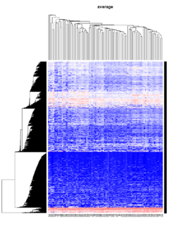
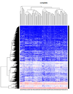
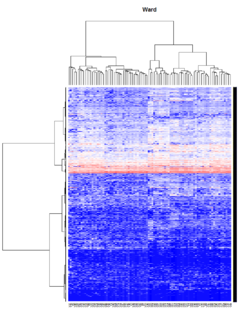
Take pomeroy data (7129 x 90) for an example:

library(gplots)

lr = read.table("C:/ArrayTools/Sample datasets/Pomeroy/Pomeroy -Project/NORMALIZEDLOGINTENSITY.txt")
lr = as.matrix(lr)
method = "average" # method <- "complete"; method <- "ward"
hclust1 <- function(x) hclust(x, method= method)
heatmap.2(lr, col=bluered(75), hclustfun = hclust1, distfun = dist,
              density.info="density", scale = "none",               
              key=FALSE, symkey=FALSE, trace="none", 
              main = method)