Bioconductor: Difference between revisions
| Line 54: | Line 54: | ||
= BiocPkgTools = | = BiocPkgTools = | ||
* [http://bioconductor.org/packages/release/bioc/html/BiocPkgTools.html BiocPkgTools]: Collection of simple tools for learning about Bioc Packages | * [http://bioconductor.org/packages/release/bioc/html/BiocPkgTools.html BiocPkgTools]: Collection of simple tools for learning about Bioc Packages | ||
* https://www.biorxiv.org/content/10.1101/642132v1 | * https://www.biorxiv.org/content/10.1101/642132v1 | ||
* [https://kevinrue.github.io/post/biocpkgtools/ GitHub Action executed as a CRON job to update the website daily] | * [https://kevinrue.github.io/post/biocpkgtools/ GitHub Action executed as a CRON job to update the website daily] | ||
Revision as of 14:23, 26 May 2020
Project
Release News
Annual reports
http://bioconductor.org/about/annual-reports/
Download stats
- See the overview vignette of BiocPkgTools
- bioconductor.riken.jp mirror in Japan
- biocpkg package in github
From the director of the project
Publications
https://www.bioconductor.org/help/publications/
Bioconductor User Support
https://support.bioconductor.org/
Mirrors
https://www.bioconductor.org/about/mirrors/
Github mirror
- https://support.bioconductor.org/p/68824/ Announcement (Update: it is dead)
Japan
Package source
Code search
http://search.bioconductor.jp/
Resource
Teaching resources from rafalab
BiocManager from CRAN
The reason for using BiocManager instead of biocLite() is mostly to stop sourcing an R script from URL which isn’t so safe. So biocLite() should not be recommended anymore.
It allows to have multiple versions of Bioconductor installed on the same computer. For example, R 3.5 works with Bioconductor 3.7 and 3.8.
On the other hand, setRepositories(ind=1:4) and install.packages() still lets you install Bioconductor packages.
BiocPkgTools
- BiocPkgTools: Collection of simple tools for learning about Bioc Packages
- https://www.biorxiv.org/content/10.1101/642132v1
- GitHub Action executed as a CRON job to update the website daily
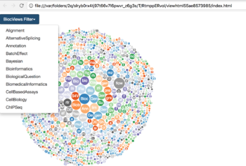
BioCExplorer
Explore Bioconductor packages more nicely
source("https://bioconductor.org/biocLite.R")
biocLite("BiocUpgrade")
biocLite("biocViews")
devtools::install_github("seandavi/BiocPkgTools")
devtools::install_github("shians/BioCExplorer")
library(BioCExplorer)
bioc_explore()
BiocViews
- Software
- AssayDomain
- BiologicalQuestion
- Infrastructure
- ResearchField
- StatisticalMethod
- Technology
- WorkflowStep
- AnnotationData
- ChipManufacturer
- ChipName
- CustomArray
- CustomCDF
- CustomDBSchema
- FunctionalAnnotation
- Organism
- PackageType
- SequenceAnnotation
- ExperimentData
- AssayDomainData
- DiseaseModel
- OrganismData
- PackageTypeData
- RepositoryData
- ReproducibleResearch
- SpecimenSource
- TechnologyData
- Workflow
- AnnotationWorkflow
- BasicWorkflow
- DifferentialSplicingWorkflow
- EpigeneticsWorkflow
- GeneExpressionWorkflow
- GenomicVariantsWorkflow
- ImmunoOncologyWorkflow
- ProteomicsWorkflow
- ResourceQueryingWorkflow
- SingleCellWorkflow
Annotation packages
- http://bioconductor.org/help/course-materials/2012/SeattleFeb2012/Annotation.pdf
- https://bioconductor.org/help/course-materials/2017/CSAMA/lectures/1-monday/lecture-04-a-annotation-intro/lecture-04a-annotation-intro.html
- Making and Utilizing TxDb Objects
- Genomic Annotation Resources Introduction to using gene, pathway, gene ontology, homology annotations and the AnnotationHub. Access GO, KEGG, NCBI, Biomart, UCSC, vendor, and other sources.
- AnnotationHub
- OrgDb
- TxDb
- OrganismDb
- BSgenome
- biomaRt
- http://genomicsclass.github.io/book/pages/bioc1_annoCheat.html
- ensembldb package
Gene centric
- AnnotationDbi: Introduction To Bioconductor Annotation Packages
library(hgu133a.db)
library(AnnotationDbi)
k <- head(keys(hgu133a.db, keytype="PROBEID"))
k
# [1] "1007_s_at" "1053_at"   "117_at"    "121_at"    "1255_g_at" "1294_at"
# then call select
select(hgu133a.db, keys=k, columns=c("SYMBOL","GENENAME"), keytype="PROBEID")

# 'select()' returned 1:many mapping between keys and columns
#     PROBEID  SYMBOL                                     GENENAME
# 1 1007_s_at    DDR1  discoidin domain receptor tyrosine kinase 1
# 2 1007_s_at MIR4640                                microRNA 4640
# 3   1053_at    RFC2               replication factor C subunit 2
# 4    117_at   HSPA6 heat shock protein family A (Hsp70) member 6
# 5    121_at    PAX8                                 paired box 8
# 6 1255_g_at  GUCA1A               guanylate cyclase activator 1A
# 7   1294_at    UBA7  ubiquitin like modifier activating enzyme 7
# 8   1294_at MIR5193                                microRNA 5193
Genomic centric
Web based
Workflow
Using Bioconductor for Sequence Data
Some packages
Biobase, GEOquery and limma
How to create an ExpressionSet object from scratch? Here we use the code from GEO2R to help to do this task.
library(Biobase)
library(GEOquery)
library(limma)

# Load series and platform data from GEO

gset <- getGEO("GSE32474", GSEMatrix =TRUE, AnnotGPL=TRUE)
if (length(gset) > 1) idx <- grep("GPL570", attr(gset, "names")) else idx <- 1
gset <- gset[[idx]]
# save(gset, file = "~/Downloads/gse32474_gset.rda")
# load("~/Downloads/gse32474_gset.rda")
table(pData(gset)[, "cell line:ch1"])
pData(gset)

# Create an ExpressionSet object from scratch
# We take a shortcut to obtain the pheno data and feature data matrices
# from the output of getGEO()
phenoDat <- new("AnnotatedDataFrame",
                 data=pData(gset))
featureDat <- new("AnnotatedDataFrame",
                  data=fData(gset))
exampleSet <- ExpressionSet(assayData=exprs(gset),
                            phenoData=phenoDat,
                            featureData=featureDat,
                            annotation="hgu133plus2")
gset <- exampleSet

# Make proper column names to match toptable
fvarLabels(gset) <- make.names(fvarLabels(gset))

# group names for all samples
gsms <- paste0("00000000111111111XXXXXXXXXXXXXXXXXXXXXXXXXXXXXXXXX",
               "XXXXXXXXXXXXXXXXXXXXXXXXXXXXXXXXXXXXXXXXXXXXXXXXXX",
               "XXXXXXXXXXXXXXXXXXXXXXXXXXXXXXXXXXXXXXXXXXXXXXXXXX",
               "XXXXXXXXXXXXXXXXXXXXXXXX")
sml <- c()
for (i in 1:nchar(gsms)) { sml[i] <- substr(gsms,i,i) }

# Subset an ExpressionSet by eliminating samples marked as "X"
sel <- which(sml != "X")
sml <- sml[sel]
gset <- gset[ ,sel]

# Decide if it is necessary to do a log2 transformation
ex <- exprs(gset)
qx <- as.numeric(quantile(ex, c(0., 0.25, 0.5, 0.75, 0.99, 1.0), na.rm=T))
LogC <- (qx[5] > 100) ||
  (qx[6]-qx[1] > 50 && qx[2] > 0) ||
  (qx[2] > 0 && qx[2] < 1 && qx[4] > 1 && qx[4] < 2)
if (LogC) { ex[which(ex <= 0)] <- NaN
exprs(gset) <- log2(ex) }

# Set up the data and proceed with analysis
sml <- paste("G", sml, sep="")    # set group names
fl <- as.factor(sml)
gset$description <- fl
design <- model.matrix(~ description + 0, gset)
colnames(design) <- levels(fl)
fit <- lmFit(gset, design)
cont.matrix <- makeContrasts(G1-G0, levels=design)
fit2 <- contrasts.fit(fit, cont.matrix)
fit2 <- eBayes(fit2, 0.01)
tT <- topTable(fit2, adjust="fdr", sort.by="B", number=250)

# Display the result with selected columns
tT <- subset(tT, select=c("ID","adj.P.Val","P.Value","t","B","logFC","Gene.symbol","Gene.title"))
tT[1:2, ]
#                  ID  adj.P.Val      P.Value        t        B    logFC Gene.symbol
# 209108_at 209108_at 0.08400054 4.438757e-06 6.686977 3.786222 3.949088      TSPAN6
# 204975_at 204975_at 0.08400054 6.036355e-06 6.520775 3.550036 2.919995        EMP2
#                             Gene.title
# 209108_at                 tetraspanin 6
# 204975_at epithelial membrane protein 2
Biostrings
- Find the location of a particular sequence. ?vmatchPattern
- https://www.bioconductor.org/help/course-materials/2011/BioC2011/LabStuff/BiostringsBSgenomeOverview.pdf
library(Biostrings)
library(BSgenome.Hsapiens.UCSC.hg19)
vmatchPattern("GCGATCGC", Hsapiens)
plyranges
http://bioconductor.org/packages/devel/bioc/vignettes/plyranges/inst/doc/an-introduction.html
Misc
Package release history
https://support.bioconductor.org/p/69657/
Search the DESCRIPTION file (eg. VariantAnnotation package) in github and the release information can be found there.
Papers/Overview
Using R and Bioconductor in Clinical Genomics and Transcriptomics 2019
