Statistics

BoxCox transformation

Finding transformation for normal distribution

Principal component analysis

R source code

> stats:::prcomp.default
function (x, retx = TRUE, center = TRUE, scale. = FALSE, tol = NULL, 
    ...) 
{
    x <- as.matrix(x)
    x <- scale(x, center = center, scale = scale.)
    cen <- attr(x, "scaled:center")
    sc <- attr(x, "scaled:scale")
    if (any(sc == 0)) 
        stop("cannot rescale a constant/zero column to unit variance")
    s <- svd(x, nu = 0)
    s$d <- s$d/sqrt(max(1, nrow(x) - 1))
    if (!is.null(tol)) {
        rank <- sum(s$d > (s$d[1L] * tol))
        if (rank < ncol(x)) {
            s$v <- s$v[, 1L:rank, drop = FALSE]
            s$d <- s$d[1L:rank]
        }
    }
    dimnames(s$v) <- list(colnames(x), paste0("PC", seq_len(ncol(s$v))))
    r <- list(sdev = s$d, rotation = s$v, center = if (is.null(cen)) FALSE else cen, 
        scale = if (is.null(sc)) FALSE else sc)
    if (retx) 
        r$x <- x %*% s$v
    class(r) <- "prcomp"
    r
}
<bytecode: 0x000000003296c7d8>
<environment: namespace:stats>

Related to SVD

Uusing the SVD to perform PCA makes much better sense numerically than forming the covariance matrix to begin with, since the formation of XX⊤ can cause loss of precision.

http://math.stackexchange.com/questions/3869/what-is-the-intuitive-relationship-between-svd-and-pca

Calculated by Hand

http://strata.uga.edu/software/pdf/pcaTutorial.pdf

Visualization based on simulated data

http://oracledmt.blogspot.com/2007/06/way-cooler-pca-and-visualization-linear.html

What does it do if we choose center=FALSE in prcomp()?

In USArrests data, use center=FALSE gives a better scatter plot of the first 2 PCA components.

x1 = prcomp(USArrests) 
x2 = prcomp(USArrests, center=F)
plot(x1$x[,1], x1$x[,2])  # looks random
windows(); plot(x2$x[,1], x2$x[,2]) # looks good in some sense

Visualize the random effects

http://www.quantumforest.com/2012/11/more-sense-of-random-effects/

Sensitivity/Specificity/Accuracy

		Predict
		1	0
True	1	TP	FN	Sens=TP/(TP+FN)
	0	FP	TN	Spec=TN/(FP+TN)
				N = TP + FP + FN + TN

• Sensitivity = TP / (TP + FN)
• Specificity = TN / (TN + FP)
• Accuracy = (TP + TN) / N

Elements of Statistical Learning

Bagging

Chapter 8 of the book.

• Bootstrap mean is approximately a posterior average.
• Bootstrap aggregation or bagging average: Average the prediction over a collection of bootstrap samples, thereby reducing its variance. The bagging estimate is defined by

[math]\displaystyle{ \hat{f}_{bag}(x) = \frac{1}{B}\sum_{b=1}^B \hat{f}^{*b}(x). }[/math]

Boosting

AdaBoost.M1 by Freund and Schapire (1997):

The error rate on the training sample is [math]\displaystyle{ \bar{err} = \frac{1}{N} \sum_{i=1}^N I(y_i \neq G(x_i)), }[/math]

Sequentially apply the weak classification algorithm to repeatedly modified versions of the data, thereby producing a sequence of weak classifiers [math]\displaystyle{ G_m(x), m=1,2,\dots,M. }[/math]

The predictions from all of them are combined through a weighted majority vote to produce the final prediction: [math]\displaystyle{ G(x) = sign[\sum_{m=1}^M \alpha_m G_m(x)]. }[/math] Here [math]\displaystyle{ \alpha_1,\alpha_2,\dots,\alpha_M }[/math] are computed by the boosting algorithm and weight the contribution of each respective [math]\displaystyle{ G_m(x) }[/math]. Their effect is to give higher influence to the more accurate classifiers in the sequence.

Classification and Regression Trees (CART)

Construction of the tree classifier

• Node proportion

[math]\displaystyle{ p(1|t) + \dots + p(6|t) =1 }[/math] where [math]\displaystyle{ p(j|t) }[/math] define the node proportions (class proportion of class j on node t. Here we assume there are 6 classes.

• Impurity of node t

[math]\displaystyle{ i(t) }[/math] is a nonnegative function [math]\displaystyle{ \phi }[/math] of the [math]\displaystyle{ p(1|t), \dots, p(6|t) }[/math] such that [math]\displaystyle{ \phi(1/6,1/6,\dots,1/6) }[/math] = maximumm [math]\displaystyle{ \phi(1,0,\dots,0)=0, \phi(0,1,0,\dots,0)=0, \dots, \phi(0,0,0,0,0,1)=0 }[/math]. That is, the node impurity is largest when all classes are equally mixed together in it, and smallest when the node contains only one class.

• Gini index of impurity

[math]\displaystyle{ i(t) = - \sum_{j=1}^6 p(j|t) \log p(j|t). }[/math]

• Goodness of the split s on node t

[math]\displaystyle{ \Delta i(s, t) = i(t) -p_Li(t_L) - p_Ri(t_R). }[/math] where [math]\displaystyle{ p_R }[/math] are the proportion of the cases in t go into the left node [math]\displaystyle{ t_L }[/math] and a proportion [math]\displaystyle{ p_R }[/math] go into right node [math]\displaystyle{ t_R }[/math].

A tree was grown in the following way: At the root node [math]\displaystyle{ t_1 }[/math], a search was made through all candidate splits to find that split [math]\displaystyle{ s^* }[/math] which gave the largest decrease in impurity;

[math]\displaystyle{ \Delta i(s^*, t_1) = \max_{s} \Delta i(s, t_1). }[/math]

• Class character of a terminal node was determined by the plurality rule. Specifically, if [math]\displaystyle{ p(j_0|t)=\max_j p(j|t) }[/math], then t was designated as a class [math]\displaystyle{ j_0 }[/math] terminal node.

R packages

• rpart
• http://exploringdatablog.blogspot.com/2013/04/classification-tree-models.html

Hierarchical clustering

For the kth cluster, define the Error Sum of Squares as [math]\displaystyle{ ESS_m = }[/math] sum of squared deviations (squared Euclidean distance) from the cluster centroid. [math]\displaystyle{ ESS_m = \sum_{l=1}^{n_m}\sum_{k=1}^p (x_{ml,k} - \bar{x}_{m,k})^2 }[/math] in which [math]\displaystyle{ \bar{x}_{m,k} = (1/n_m) \sum_{l=1}^{n_m} x_{ml,k} }[/math] the mean of the mth cluster for the kth variable, [math]\displaystyle{ x_{ml,k} }[/math] being the score on the kth variable [math]\displaystyle{ (k=1,\dots,p) }[/math] for the lth object [math]\displaystyle{ (l=1,\dots,n_m) }[/math] in the mth cluster [math]\displaystyle{ (m=1,\dots,g) }[/math].

If there are C clusters, define the Total Error Sum of Squares as Sum of Squares as [math]\displaystyle{ ESS = \sum_m ESS_m, m=1,\dots,C }[/math]

Consider the union of every possible pair of clusters.

Combine the 2 clusters whose combination combination results in the smallest increase in ESS.

Comments:

1. Ward's method tends to join clusters with a small number of observations, and it is strongly biased toward producing clusters with the same shape and with roughly the same number of observations.
2. It is also very sensitive to outliers. See Milligan (1980).

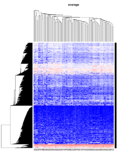
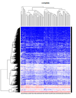
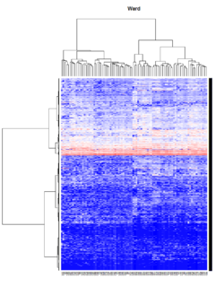
Take pomeroy data (7129 x 90) for an example:

library(gplots)

lr = read.table("C:/ArrayTools/Sample datasets/Pomeroy/Pomeroy -Project/NORMALIZEDLOGINTENSITY.txt")
lr = as.matrix(lr)
method = "average" # method <- "complete"; method <- "ward"
hclust1 <- function(x) hclust(x, method= method)
heatmap.2(lr, col=bluered(75), hclustfun = hclust1, distfun = dist,
              density.info="density", scale = "none",               
              key=FALSE, symkey=FALSE, trace="none", 
              main = method)

Mixed Effect Model

• Paper by Laird and Ware 1982
• John Fox's Linear Mixed Models Appendix to An R and S-PLUS Companion to Applied Regression. Very clear. It provides 2 typical examples (hierarchical data and longitudinal data) of using the mixed effects model. It also uses Trellis plots to examine the data.
• Chapter 10 Random and Mixed Effects from Modern Applied Statistics with S by Venables and Ripley.
• (Book) lme4: Mixed-effects modeling with R by Douglas Bates.
• (Book) Mixed-effects modeling in S and S-Plus by José Pinheiro and Douglas Bates.

Entropy

Entropy is defined by -log2(p) where p is a probability. Higher entropy represents higher unpredictable of an event.

Some examples:

• Fair 2-side die: Entropy = -.5*log2(.5) - .5*log2(.5) = 1.
• Fair 6-side die: Entropy = -6*1/6*log2(1/6) = 2.58
• Weighted 6-side die: Consider pi=.1 for i=1,..,5 and p6=.5. Entropy = -5*.1*log2(.1) - .5*log2(.5) = 2.16 (less unpredictable than a fair 6-side die).

When entropy was applied to the variable selection, we want to select a class variable which gives the largest entropy because this variable is most discriminative and it gives most information gain.

Why is picking the attribute with the most information gain beneficial? It reduces entropy, which increases predictability.