Arraytools: Difference between revisions
| Line 496: | Line 496: | ||
=== DNA Methylation === | === DNA Methylation === | ||
* [https://www.illumina.com/Documents/products/appnotes/appnote_dna_methylation_analysis_infinium.pdf Comprehensive DNA Methylation Analysis on the Illumina® Infinium® Assay Platform]. [https://en.wikipedia.org/wiki/Epigenetics Epigenetic analysis]. | |||
'''N.B.''' There is an issue (IlluminaHumanMethylation450k.db is deprecated) with methylation 450k annotation in version 4.5 beta (R 3.2.x):( So instead of choosing to use the Bioconductor package to annotate data, users need to download the annotation file <GPL13534-11288.txt> from [http://www.ncbi.nlm.nih.gov/geo/query/acc.cgi?acc=GPL13534 NCBI-GEO] and use the file to do annotation. In the dialog, choose Unique ID = Col 1, Gene symbol = Col 22 UCSC_RefGene_Name, GenBank Accession = Col 23 UCSC_RefGene_Accession. | '''N.B.''' There is an issue (IlluminaHumanMethylation450k.db is deprecated) with methylation 450k annotation in version 4.5 beta (R 3.2.x):( So instead of choosing to use the Bioconductor package to annotate data, users need to download the annotation file <GPL13534-11288.txt> from [http://www.ncbi.nlm.nih.gov/geo/query/acc.cgi?acc=GPL13534 NCBI-GEO] and use the file to do annotation. In the dialog, choose Unique ID = Col 1, Gene symbol = Col 22 UCSC_RefGene_Name, GenBank Accession = Col 23 UCSC_RefGene_Accession. | ||
Revision as of 11:28, 22 February 2023
Wiki for BRB-ArrayTools . See also my Wiki for BRB-SeqTools.
Features
Import from multiple data types
Expression data, Illumina methylation data, Copy number data (CGH-Tools), RNA-Seq count data processed through Galaxy web tool.
Sophisticated statistical analysis tools
Class comparison for differential expression, class prediction, graphical 2d and 3D interactive plots, gene set analysis, and more.
Comprehensive biological annotations
Gene ontology, pathways, protein domain, broad msigdb, lymphoid signatures, experimentally verified transcription factor targets, computationally predicted microRNA targets.
ArrayTools/Genelists/Cgap
                    /Lymphoid
                    /MicroRNA/experimentally_verified_human
                             /experimentally_verified_mouse
                    /Protein_domain/Human_domain_Pfam
                                   /Human_domain_SMART
                                   /Mouse_domain_Pfam
                                   /Mouse_domain_SMART
                    /Transcription_factor/Predicted_Human (eg AR_MA0007.2, search by "MA0007")
                                         /Predicted_Mouse
                                         /TRED_Human
                                         /TRED_Mouse
                    /User
ArrayTools/Pathways/Input
                   /KEGGHD
                   /Output/Biocarta
                          /KEGG
Screenshots
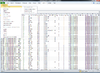 BRB-ArrayTools graphical user interface

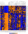 Heatmap and dendrogram generated from the Pomeroy sample dataset.

 Interactive MDS plot of samples from running the multidimensional scaling analysis on the Pomeroy dataset.

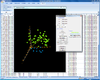
 Interactive 3D scatterplot of genes on the Pomeroy dataset.

X-axis is from array 'Brain_MD_1', y-axis is 'Brain_MD_2' and z-axis is 'Brian_MD_3'.
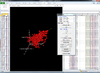
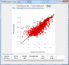 Interactive 2D scatterplot of samples with gene annotation from a selected gene using right click menu.

The right click menu gives an option to highlight up/down-regulated genes, export gene list, copy plot to clipboard, highlight genes in gene set, link genes among plots and change properties of the plot like title, point size, color of points, fold change threshold for up/down regulated genes.
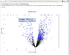 Interactive volcano plot from the output of running a class comparison tool.

When you move mouse over a gene (point), the gene unique ID and/or symbol will be popped up.
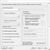 Class Prediction tool

And the option dialog.

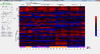 Dynamic Heatmap Viewer

Note that the center and scaling options in "Analysis Options" block in the dialog only affects the heatmap. The options only affect the heatmap but they do not affect the clustering. That is, the clustering was run using the original data (log intensities/ratios) without further transformation. This can be verified by running the analysis and varying the options 'center and scaling', 'center' or 'None'. The clustering dendrograms should be the same.
The same plot when we zoom in to a subset of genes (use PC mouse to select a range of genes) is

Below is the VBA main and options dialogs from the ArrayTools.
 ,
, 
 HTML output of running the class comparison analysis.

 HTML output containing SAM plot from running the significance of microarray analysis.

 HTML output of running the class prediction analysis.

 HTML output of running the survival risk analysis.

 Result of sample size analysis.

FAQs
General
Error in installation
If you see the following error (The installed version of the application could not be determined. The setup will now terminate), try to move the installer to your local drive.

NIH users
Please install the Privilege Manager software and install the BRB-ArrayTools by using the elevated permissions with your account (right click the installer and select the elevated privilege option). Do not let IT to use their administration account to install the BRB-ArrayTools for you!

How to install BRB-ArrayTools if you have 64-bit MS-Office?
There is no difference in terms of the installation.
After installation, I did not find the BRB-ArrayTools in Windows > Start > All Programs.
Check EXCEL. ArrayTools and CGHTools are under the Excel menu of Addon.
If you only see 'CGHTools' under the ADD-INS, it means you have skipped/ignored the screen of an instruction to the user. See the next item.
After installation, I did not find the BRB-ArrayTools in Excel (Office 2016/365) Add-ins/ribbon
- Click on “File->Options”. Select “Trust Center” in the left box, click on “Trust Center Setting…” and a new dialogue will pop up. In the new dialogue, select “Macro settings” and make sure “Trust access to the VBA project object model” is selected.
- Go to “File->Options”. Click on “Add-ins” on the left, and click on the “Go…” button. Click on the “Browse” Button, browse for your ArrayTools installation folder (default C:\Program Files (x86)\ArrayTools\) Excel\ArrayTools.xla, and click on OK. Click “OK” in the “Add-ins” Dialogue.
- Close Excel and then restart Excel.
If the "Add-ins" tab appears, please click on it to see if ArrayTools is there. If the "Add-ins" tab still cannot be found, you can go to the folder (C:\Program Files (x86)\ArrayTools\Excel) containing the "ArrayTools.xla" file, double-click to open the file, and the add-ins will be loaded as you have seen.
After open Excel, what options I need to do in Excel before using BRB-ArrayTools
Proceed the following no matter the BRB-ArrayTools' instruction to users is on screen or not.
(Office 2007) Excel -> Home -> Options -> Trust Center -> Trust Center Settings -> Macro Settings -> Check 'Trust access to the VBA project object model' -> OK. Restart Excel.
(Office 2010 & 2013) Excel -> File -> Options -> Trust Center -> Trust Center Settings -> Macro Settings -> Check 'Trust access to the VBA project object model' -> OK. Restart Excel.
Once Excel is restarted, it will ask to enter the email address you have registered with the BRB-ArrayTools. Then click the 'Activate' button. An Rserve app will be opened and sitting on the Windows' task bar. Do not worry about it. It will be used by BRB-ArrayTools and will be closed when the Excel is closed.
Users without Admin Privilege
- log in as the administrator and set up BRB-ArrayTools in Excel. Plus, I had to enter my email address for activation.
- log in as standard user and click the Go button for Manage Excel add-ins. Since BRB-ArrayTools add-in was still not showing up in the dialog box, I had to manually add it by clicking on the Browse button.
Foreign language users, decimal mark, thousands separator
Below are some of the recommendations we typical make to foreign language users: 1: Please, make sure that the regional language settings on your machine to the "English". You can do so by going to the Control Panel -> Regional and Language Options and choose English. 2: Windows Start > Programs > Microsoft office > Microsoft Office Tools ->Microsoft Office 20XX language settings. Make sure that the "primary editing language" is "English". If the "Primary editing language" is not "English", please change it to "English" and then re-boot your machine.
If we don't want to change the setting to "English". The trick was to: in Excel Add-Ins, look for the add-ins among folders (in the German version: Durchsuchen) and to folder programs v 64 bit. Then it finds ArrayTools there, go to subfolder Excel and there it finds the Add-in. Otherwise it was invisible.
And in Excel Options -> Advanced -> Change decimal to dot . and thousands to comma. See Change the character used to separate thousands or decimals.
Java installation
Note that the current version of Java does not work well with clusterLG.exe program on Windows 7 OS. When you run the Gene Cluster 3.0, an error screen will show up saying Error starting Java. Please make sure that javaw.exe is in your path. when you click one of the linkage method buttons (this will trigger the execution). Continue to read.
When Java run time library is installed, it will add C:\ProgramData\Oracle\Java\javapath to the environment variable PATH. Within this directory, there are 3 symbolic links java, javaw and javaws. They point to
 Directory of C:\ProgramData\Oracle\Java\javapath

08/21/2015  12:39 PM    <DIR>          .
08/21/2015  12:39 PM    <DIR>          ..
08/21/2015  12:39 PM    <SYMLINK>      java.exe [C:\Program Files (x86)\Java\jre1.8.0_60\bin\java.exe]
08/21/2015  12:39 PM    <SYMLINK>      javaw.exe [C:\Program Files (x86)\Java\jre1.8.0_60\bin\javaw.exe]
08/21/2015  12:39 PM    <SYMLINK>      javaws.exe [C:\Program Files (x86)\Java\jre1.8.0_60\bin\javaws.exe]
We can check the current version of Java by running
java -version
The Java I am using is version 8 update 60 (build 1.8.0_60-b27, 8/21/2015) available from http://www.java.com/en/download/win10.jsp. If I manually download the file, the file name is called JavaSetup8u60.exe.
One possible solution is to let VBA to get Java path and then pass/add the java path to the <EisenCluster/RunEisenCluster.bat> file before calling clusterLG.exe.
R installation directory
The default installation location for R software is OK. But if you use some other R packages like Rcpp, it is recommended to install R to C:\R folder.
Caution: Do not open another instance of R when BRB-ArrayTools is working. This may make R packages installation/update impossible.
R: Unable to install packages
If you see the following message
Error in install.packages(update[instlib == l, "Package"], l, repos = repos,  :
  unable to install packages
you want to check if you have a full privilege on R or R-x.x.x folder.
- Open Windows Explorer (Win + e), go to C:\Program Files
- Right click the 'R' folder ('R' folder is a parent of 'R-x.x.x' folder, so selecting it is better than selecting 'R-x.x.x'), choose 'Properties'
- Click 'Security' > 'Advanced'
- Click 'Owner' and select from the list to make sure the current user is the owner.
- Click OK button multiple times to finish the change.
Error: package 'X' required by 'Y' could not be found
The 'X' and 'Y' could be anything from CRAN or Bioconductor repository. One direct way to tackle the error is to open an R gui and install the missing packages manually. For example, if 'X' is 'preprocessCore' (a package in Bioconductor).
source("http://bioconductor.org/biocLite.R")
biocLite("preprocessCore")
If the missing package is from CRAN, we can use install.packages() function directly.
Can I upgrade R or install multiple versions of R?
Installing multiple versions of R is OK provided you know some details described below.
Each version of BRB-ArrayTools has been tested with a certain version of R. So there may be a compatibility problem with certain functions used in the code if you decide to a non-default version of R.
- BRB-ArrayTools (before v4.3.0) requires StatconnDCOM which means the following conditions have to be satisfied:
- R needs to registered in the Windows's registry (it should be done if you accept all default options when R was installed).
- The R package 'rscproxy' has to be installed under the library folder the registered R. It cannot be installed under user's Document's folder as other R's packages.
- BRB-ArrayTools (from v4.3.0) requires Rserve package. That means
- Run install.packages("Rserve", repos="https://cran.rstudio.com") in an R console.
- Open Window's file manager. Check whether the Rserve package is installed under C:\Program Files\R\R-X.Y.Z\R\library folder Document\R\win-library\X.Y folder where X is the major, Y is the minor and Z is the patch number of R version.
- (If Rserve package is located under Document\R\win-library\X.Y) Rserve.exe from Documents\R\win-library\X.Y\Rserve\libs\i386 and Documents\R\win-library\X.Y\Rserve\libs\x64 subfolder has to be copied to C:\Program Files\R\R-X.Y.Z\bin\i386 and R\bin\x64 folder
- (If Rserve package is located under C:\Program Files\R\R-X.Y.Z\library) Rserve.exe from C:\Program Files\R\R-X.Y.Z\library\Rserve\libs\i386 and C:\Program Files\R\R-X.Y.Z\library\Rserve\libs\x64 subfolder has to be copied to C:\Program Files\R\R-X.Y.Z\bin\i386 and R\bin\x64 folder where X is the major, Y is the minor and Z is the patch number of R version.
Understand above will allow you to use a non-default version of R with BRB-ArrayTools.
If you want use the latest version of R for your own analysis but still use the default version of R in BRB-ArrayTools, keep reading. First, install the latest version of R as usual. Then install again the full-version of BRB-ArrayTools and R included in the BRB-ArrayTools installer. This will possibly install another version of R and register it in the Windows's registry. Now you can enjoy both versions of R as you want. The idea is when you install R, it will by default register R, but this behavior can break the setting for R to be used by BRB-ArrayTools. Once you install BRB-ArrayTools again, it will install a version of R that BRB-ArrayTools has tested and not erase any other versions of R you already have.
How to upgrade Bioconductor
For example, my bioc is 2.12 which was first installed when I use R 3.0.1. But bioc 2.13 is the current version when R 3.0.2 was used. When I need to install a new package from bioc, the new package may requires a new version of bioc package.
source("http://bioconductor.org/biocLite.R")
biocLite("BiocUpgrade")
This command will upgrade all currently installed bioc related packages. But it seems it will install lots of other bioc packages I don't need.
My institute is using a proxy server. So how do I do with BRB-ArrayTools
See the message on BRB-ArrayTools message board. Essentially we need to create a Windows environment variable http_proxy with a value like
http://myproxy:myport
OR
http_proxy=http://username:[email protected]
OR
http_proxy=http://username:[email protected]:81
RExcel-statconnDCOM gave an error
Please upgrade BRB-ArrayTools to v4.3.x where Rserve has replaced statconnDCOM.
Rserve
Since version 4.3.0, BRB-ArrayTools started to use Rserve as a media for the communication between R and Excel. When Rserve is required, an R window will be pop up. This R window has a blue icon on the Windows' taskbar. If you accidentally close it, it will be automatically popped up when it is needed.
See my Rserve wiki page.
Biological replciates vs technical replicates
When the same type of organism is grown/treated under the same conditions. Or if you repeat the experiment, and keep everything the same, it is a biological replicate.
When the exact same sample (after all preparatory techniques) is analyzed multiple times, it is called the technical replicates.
Reducing multiple probes/probe sets to one per gene symbol
For affymetrix data, in the 'Refilter, normalize and subset the data' - 'Gene subsets' dialog, it provides two options to reduce the number of genes in gene expression.
- Use the most variable probe (set) measured by IQR across arrays
- Use the maximally expressed probe (set) measured by average intensity across arrays
x <- matrix(1:60, nr=10); x[1, 2:3] <- NA; x
rownames(x) <- c(rep("b", 2), rep("c", 3), rep("d", 4), "a")
res <- sapply(split(1:nrow(x), rownames(x)),
           function(i) x[i,, drop=F][which.max(rowSums(x[i, , drop=F], na.rm = TRUE)),])
t(res)
  [,1] [,2] [,3] [,4] [,5] [,6]
a   10   20   30   40   50   60
b    2   12   22   32   42   52
c    5   15   25   35   45   55
d    9   19   29   39   49   59

Average the replicate spots within an array
In the 'Refilter, normalize and subset the data' - 'Spot filter' dialog, the checkbox of 'Average the replicate spots within an array' will compute the average on the INTENSITY level. This is different from the way other analyses are doing.
For example, if two spots (same gene ID) have log2 expression values a and b, then the average log2 expression value will be log2((2^a + 2^b)/2).
Windows Security Warning
The message pops up when an R script was run in a parallel fashion on Windows OS. See here. Note that parallel computing is still working even the 'Cancel' button was chosen.
Importing
Summary
Data import wizard
- Affy Cel file
- Affy Gene ST array including Affymetrix human/mouse/rat Clariom S/D arrays (HT). Alternatively choose General Importer and pick Human Clariom D Array from the dropdown list. PS. it is OK to ignore the message that ID column does not have “_” at the end of probeset name. Also Clariom S and D arrays have different annotations. If you use the Affymetrix Gene ST Array Importer in ArrayTools, it will take care of annotations automatically.
- Affy probe-set summary
- RNA-Seq data from Galaxy; more specifically the FPKM value (see http://linus.nci.nih.gov/~brb/GalaxyDoc.pdf and an example of <genes.fpkm_tracking> file output from cuffdiff program (GSE32038)
- Agilent dual channel data
- Agilent single channel data
- Genepix dual channel data
- Genepix single channel data
- Illumina single channel data
- mAdb archive data
- Illumina methylation data
General format importer
When generating the txt files of expression or gene identifiers or experiment descriptor from R, remember to choose the option row.names = FALSE.
require(tibble)
foo_at <- function(x) {
  # utility to create BRB-ArrayTools expression matrix file
  # It will add a column 'Id' in front of the matrix 'x'
  cbind(tibble(Id=rownames(x)), as_tibble(x))
}
# Suppose the rows of 'x' contain the gene/feature ID
write.table(foo_at(someMatrix),
            file = "expression.txt",
            quote = F, row.names = F, sep = "\t")
NCBI GEO GDS
ArrayTools will download 3 files (GPLXXX.annot.txt, GDSXXX.txt and Readme_GDSXXX.txt). The <Experiment Descriptor file.txt> file is generated from the soft file (ParseGEOProjectFile() function).
The download command for the soft file (including expression and experiment descriptor) is wget -N -nd ftp://ftp.ncbi.nih.gov/pub/geo/DATA/SOFT/GDS/GDSGDSNumber.soft.gz. The gz file (eg GDS1344.soft.gz) contains a soft file (eg GDS1344.soft) where the soft extension will be renamed to .txt.
The GPL file is downloaded from ftp://ftp.ncbi.nih.gov/pub/geo/DATA/annotation/platforms/Dataset_platform.annot.gz.
The Readme file is only for the record and seems not to be used anymore.
NCBI GEO GSE
The importer will ask whether we want to do the log transformation. It's not clear what to do. However, GEO2R has a special way to guess this. For example in GSE22093, it use the following way:
gset <- getGEO("GSE22093", GSEMatrix =TRUE, getGPL=FALSE)
if (length(gset) > 1) idx <- grep("GPL96", attr(gset, "names")) else idx <- 1
gset <- gset[[idx]]

ex <- exprs(gset)

# log2 transform
qx <- as.numeric(quantile(ex, c(0., 0.25, 0.5, 0.75, 0.99, 1.0), na.rm=T))
# On an already log2 transformed data such as GSE22093, qx is
# [1] -2.994992  6.531386  8.156300  9.475783 13.930978 18.619087
# On an intensity-based data such as GSE7810, qx is
# [1]     0.00    36.20   122.80   527.80 10338.15 34114.50

LogC <- (qx[5] > 100) ||
          (qx[6]-qx[1] > 50 && qx[2] > 0)
if (LogC) { ex[which(ex <= 0)] <- NaN
  ex <- log2(ex) }
source("https://bioconductor.org/biocLite.R")
biocLite("GEOquery")

  require(GEOquery)
  # VBA
  GSA <- getGEO("GSE22631", GSEMatrix = F)  # by default GSEMatrix = TRUE
  DataType <- Meta(GSE)$type
  NumPlatform <- length(Meta(GSE)$platform_id)
  PlatformID <- ChipName <- Meta(GSE)$platform_id # eg GPL1435, only be used if there are > 1 platforms.
  # R
  gse <- getGEO("GSE22631") # fetch from ftp://ftp.ncbi.nlm.nih.gov/geo/series/GSE22nnn/GSE22631/matrix/GSE22631_series_matrix.txt.gz
  data <- gse[[1]]
  exp <- exprs(data)
  if (as.logical(ApplyLog))  exp <- log2(exp)
  ...
It will create GeneID.txt, ExpDesc.txt and TempFolder/GSMXXXXXX.txt files where
- GeneID.txt - fData(data)
- ExpDesc.txt - complicated calculation from pData(data)
To get the phenotype data,
gse <- getGEO("GSE68465")   # it won't work by using filename="GSE68465_family.soft.gz"
show(gse)
pheno <- pData(gse[[1]])
dim(pheno)
#  462  63
data <- exprs(gse[[1]])
data <- log2(data)

gid <- fData(gse[[1]])
colnames(gid)
#  [1] "ID"                               "GB_ACC"                           "SPOT_ID"
#  [4] "Species Scientific Name"          "Annotation Date"                  "Sequence Type"
#  [7] "Sequence Source"                  "Target Description"               "Representative Public ID"
# [10] "Gene Title"                       "Gene Symbol"                      "ENTREZ_GENE_ID"
# [13] "RefSeq Transcript ID"             "Gene Ontology Biological Process" "Gene Ontology Cellular Component"
# [16] "Gene Ontology Molecular Function"
colnames(gid)[c(1,2,11,12)]
# [1] "ID"             "GB_ACC"         "Gene Symbol"    "ENTREZ_GENE_ID"
anno[, 3] <- gsub("///.+", "", anno[, 3])  # Keep only the first one when multiple appears
anno[, 4] <- gsub("///.+", "", anno[, 4])  # eg DDR1 /// MIR4640 will keep DDR1
RNA-Seq count data importer
NanoString count data
Manufacturer http://www.nanostring.com/
nCounter® Expression Data Analysis Guide
Use General Importer
GEO repository: https://www.ncbi.nlm.nih.gov/gds/?term=nanostring
- R package: NanoStringNorm
- Bioconductor packages: NanoStringQCPro , NanoStringDiff
- NanoStriDE: normalization and differential expression analysis of NanoString nCounter data
GDS from GEO (Gene Expression Omnibus)
- If there is a GDS number, use GEO importer to import data (eg GDS1348). Expression data, experiment description and gene identifiers will be created automatically. BRB-AT downloads GDSxxx.soft.gz file from this ftp/retired dataset and GPL files from ftp. The <GDSxxxx.soft> file can be used to create <Experiment Descriptor file.txt> and <GDS1348.txt> files for BRB-AT. Note that dataset with GDS number contains experiment info. Individual Experiment (GSMxxxx) does not have experiment info. We can browse all GDS datasets from this ftp link.
- The DataSet Browser (GEO -> Series -> DataSets) provides a table of curated datasets sorting by the GDS number. Currently it has 3848 dataset records. Each GDS does not have its own website though and the latest GDS 5093 has a GSE number on 2014/8/13. Since each GDS also a GSE number, we can compare the importing results from BRB-ArrayTools.
- A GDS may be only a subset of GSE series. For instance, GDS 5091 has 7 samples but its GSE 47516 series contains GDS 5089, GDS 5090, GDS 5091.
- It is possible to view the 'Experiment descriptors' for GDS data without downloading the gene expression data. To see that, click the 'Sample subsets' tab in the GDS browser.
- A list of all GDS data can be found on GEOmetadb website (not sync with GEO).
GSE from GEO
Note:
- BRB-ArrayTools v4.5.0 provides a new tool to import GSE data using the Bioconductor GEOquery package. However, the data type GSE29135 is categorized as “Non-coding RNA profiling by array” instead of the type Expression profiling by array or gene expression array-based, it was not considered as expression arrays.
- GSE series can be obtained from http://www.ncbi.nlm.nih.gov/geo/index.cgi and choose Browse Content|Series.
- Some GSE data has a GDS number too. For example GDS 2875 has a GSE 7810. To find the GDS number, we can use one of the following 2 ways:
- Click BioProject PRJNA 100031 -> Project Data, GEO DataSets Links 2 -> GDS 7810.
- Select gds in GEOmetadb page. Click Select Field 'GSE contains GSE7810' and hit the Search button. Some new data in GEO may not appear in the GEOmetadb website though.
The information provided below is for BRB-ArrayTools version up to v4.4.x.
You can go to GEOmetadb at http://gbnci.abcc.ncifcrf.gov/geo/ to extract sample information of your interest. This GEO microarray search tool makes access to metadata associated with NCBI GEO samples, platforms and datasets much more feasible.
Let us take GSE29135 for example. Please try the following to extract sample information for this dataset:
- Go to http://gbnci.abcc.ncifcrf.gov/geo/ .
- Click on “GSE Search” link below "GEOmetadb Web Interface", and you will be directed to the GSE search page.
- Under "Select Filed:", select "GSE Acc" for the left drop-down list, type "29135" in the right box and then click on "search" button.
- Click on “25983” in the column “ID”. In the new page of “View GSE Details”, click on “Show GSM” button. This will show all the GEO GSM records of GSE29135 extracted from GEO.
- In this case, information of “GSM Acc” and “Title” from the table seems to be useful. To extract them, you can go click on “Display Options” and put only “GSM Acc” and “Title” fields in “Selected Fields” by removing the others using the left arrow button. Then click on “Change” button on the top right.
- Click on “Download Results” and save the .csv file. It contains three columns in this example, that is, ID, GSM Acc and Title. You may delete ID column manually since it is useless. Also, please replace the comma delimiter with the tab delimiter by using Notepad++ (a text editor for free downloading). By cleaning up the table and adding column names, the processed table should look like this:
Experiment Names  Patient ID Stage     Subtype
GSM712531         101        IA        AD
GSM713230         107        Ib        AD
GSM713231         112        IA        Broncho-alveolar
GSM713236         175        IB        AD
GSM713237         147        IB        AD
…
7. Save this table as .txt file. And this file can be used the experimental descriptor during importing.
If you are interested in other characteristics of the data set, you may go each GSM link and check them out.
As for the gene information, please go to the platform GPL8179 page of GSE29135 at http://www.ncbi.nlm.nih.gov/geo/query/acc.cgi?acc=GPL8179. You may take a look at GPL8179_humanMI_V2_R0_XS0000124-MAP.txt.gz for information of your interest.
Other types from GEO
- If there is raw data, we can try to import them with data import wizard (eg GSE18170). We can use SOURCE to annotation data using 'Symbol' as the lookup key. Select 'Mouse' as the organism.
- If there is no raw data, we can use Serial matrix file with General Importer (eg GSE33403). Download GPL10481_family.soft.gz file and Extract it. Open the file in EXCEL. Copy the cells on rows from126 to 45346 and columns from A to I. Paste them to a new Workbook and save it in a tab-delimited format file called <SeriesMatrix.txt>. Download GSE33403_series_matrix.txt.gz file and extract it. Open it in EXCEL. Copy the data on rows from 75 to 45295 and columns from A to AN. Paste them to a new Workbook and save it in a tab-delimited format file called <GeneID.txt>.
Affymetrix normalization
- RMA/Robust Multi-array Average
- Exploration, Normalization, and Summaries of High Density Oligonucleotide Array Probe Level Data Biostatistics, Rafael A. Irizarry 2003
- https://www.rdocumentation.org/packages/affy/versions/1.50.0/topics/rma. Note that this expression measure (RMA) is given to you in log base 2 scale. This differs from most of the other expression measure methods.
- Background correction + Quantile normalization + Summarization (Tukey's median polish)
- http://www.math.usu.edu/jrstevens/stat5570/1.4.preprocess_4up.pdf
- http://master.bioconductor.org/help/course-materials/2009/GenentechNov2009/Module2/module2-affy-preprocess.pdf
- http://rmaexpress.bmbolstad.com/
- MAS5: The numbers on an ExpressionSet created with MAS 5.0 are on the same scale as the signal intensities and range from 100 to several thousand. Normally a threshold of 500 is used to decide if the gene is expressed at all. Amount of mRNA is roughly proportional to the measure.
- GCRMA: like RMA, GCRMA are on a log2 scale. Values range from 2 to 15 or so. Amount of mRNA is roughly 2x, where x is the expression value.
Control probes
Start with AFFX. See https://www.biostars.org/p/378071/
Multiple chips (hgu133a and hgu133b)
GSE4922 contains two different array platforms (hgu133a and hgu133b). Starting from ArrayTools v4.1 our software does not support the importing of multi-chips any more. Therefore you cannot directly import all the data into BRB-ArrayTools to create one project with two different chips. However, you could import the data into ArrayTools as two different projects and output the normalized data for each project. Then you can manually combine the two output data files and re-import into BRB-ArrayTools as one project. Here is what you can do,
- Use Data Import Wizard to import the CEL files for hgu133a and hgu133b chips separately to create two projects.
- Open each project and then use the "Export 1-color data to R" plug-in (click on "ArrayTools -> Plugins -> Export 1 color data to R") to output your normalized data file along with the GeneId file.
- Under Excel, combine the normalized output files ("NORMALIZEDLOGINTENSITY.txt") from two projects. Add sample names in the first row and Probe Set Ids in the first column. Save this combined data file. Then combine the two "GENEID.txt" files manually to create one Gene ID file.
- Open Excel, Click on "ArrayTools -> Import data -> General format importer" to import the combined data file. Select your data as "Single-channel", "Affymetrix probeset-summary data". For the chip type, because your data contain probe sets from both hgu133a and hgu133b, almost all of which were included in the hgu133plus2 chip, you can just pick the hgu133plus2 as your chip type. Alternatively, if you do not wish to do this, you can check "I would like to use my own gene identifiers file rather than the one from bioconductor" and use the combined Gene ID file (done in step 3) for annotation.
- At the filter and normalization step, it is VERY IMPORTANT that you need to uncheck all the spot filter and normalization options, because your "raw" data file comes from already normalized data in two different projects. You do not want to re-run normalization. You can keep the options in "Gene filter" tab.
- At the end you can run annotation as your choice.
PrimeView importing failed on v4.3.0 beta1 (R 2.14.x)
- Go to http://www.bioconductor.org/packages/2.11/data/annotation/html/primeviewcdf.html and click on the link for the windows binary package "primeviewcdf_2.11.0.zip" and download the zipped package.
- Unzip the downloaded package and put the entire package folder "primeviewcdf" under your R2.14.2 library folder (default C:\Program Files\R\R-2.14.2\library).
However, you cannot run Affymetrix annotation using bioconductor annotation packages at the end of importing, because the annotation package for primeview array is not available at bioconductor. Another commonly use annotation database, SOURCE, has also been down these days. Instead you need to import your own annotation into BRB-ArrayTools. Here is what you can do,
- Download the primeview annotation file in CSV format from Affymetrix website (https://www.affymetrix.com/user/login.jsp?toURL=/support/file_download.affx?onloadforward=/analysis/downloads/na32/ivt/PrimeView.na32.annot.csv.zip).
- Open the CSV format file in Excel and then save it as a tab-delimited .txt file.
- Import your data in CEL file format into BRB-ArrayTools through Data Import Wizard. During importing, you need to check the option "Import your own identifiers file to annotate your data" at the "Probe Set Id options" page, and then Click on "OK". At the next dialog form you need to select the radio button "The identifiers are stored in a separate file" and browse for the tab-delimited file you just saved. The head line # for this file is 25. Then you need to select the corresponding gene identifiers column headers. You need to check the box "Annotate the project with these gene ids, instead of using the data from SOURCE database" before proceeding to the next page.
Affymetrix miRNA 2.0, 3.0 or 4.0
For Affymetrix miRNA 2.0 array GPL14613, eg GSE43592 (not for 3.0 array, GPL16384 search GEO by keywords miRNA 3_0, since there is no cdf package), you can import the data in CEL file format into BRB-ArrayTools through the CEL file importer (from Data Import Wizard). For miRNA 2.0 and 3.0 arrays, an alternative way is to use the Affymetrix expression console software to pre-process/normalize the CEL file data and obtain a tab-delimited probe-set summary data file to be imported into BRB-ArrayTools using the General format importer. The Affymetrix expression console software can be downloaded at the Affymetrix website. Unlike what we do for the regular gene expression chips, BRB-ArrayTools currently does not support the generation of annotation information based on the microRNA ID (so gene set analysis cannot be run).
For now, the CSV format annotation file provided by Affymetrix can be opened in Excel and then saved as a tab-delimited .txt file, which can be used as a "Gene Identifiers" file for BRB-ArrayTools. When you import your data file into BRB, you can choose to "use your own gene ID file for annotation" and select the "Transcript Id (Array Design)" as the microRNA Id column header. Although we do not directly provide any annotation tools for miRNA data, if you run some particular analyses such as class comparison, there will be a hyperlink associated with the microRNA Id in your html output result file. By clicking on this link, you can be directed to the miRBase website with the annotation information associated with this particular microRNA Id.
Agilent miRNA
The arrays in the GSE41874 series were scanned by an Agilent scanner and data were extracted by the feature extraction software, therefore the raw data files in this series are in the exactly same format as the Agilent dual-channel .txt files. You can use Data Import Wizard and choose "Agilent dual-channel data" to import the data into BRB-ArrayTools. However, you need to select the following options:
- At the GeneID dialog form page, select the "GeneName" as the miroRNA ID, and select "None" as the Gene Symbol
- At the spot filtering step, use dye swap for all the arrays, as Cy5 was used as the reference for all arrays
- Also, please bear in mind that only some analysis tools can be used for this set of data, because annotation cannot be conducted on microRNA array data in BRB-ArrayTools. For instance, you can run class comparison and clustering with this data set, but cannot perform gene set enrichment analysis.
Although annotation is not provided, at the end of class comparison, the significant microRNAs can be hyperlinked to the mirBase if you want to see detailed annotation of any particular microRNAs.
Gene ST 1.1 (or other than 1.0), Exon ST, or Affymetrix .cel files without cdf packages from Bioconductor
You will need to install Affymetrix Expression Console. Here is the link of Affymetrix Expression Console download website. http://www.affymetrix.com/browse/level_seven_software_products_only.jsp?productId=131414&categoryId=35623#1_1
Here is the link where you could download Affymetrix Expression Console (64bit).
Take the mouse Gene 1.1 ST-array as an example on how to use the Expreesion console to convert .cel files into .txt files and then import .txt files into ArrayTools.
- Before downloading the Affymetrix expression console, you need to register at Affymetrix website. After downloading and installing the software, open Affymetrix expression console, name the profile and set a library path by clicking "Edit -> Set library path";
- After you download and install the software, please open it and then download both the library file and annotation file for mogene 1.1 ST-array in the software(File->Download Library Files and File->Download Annotation Files).
- After you download both files, you could click on "File" -> "New study" to open the Affymetrix study window. Click on "Add intensity files" to browse for the CEL files of your interest. Click on "Run analysis".
- When the analysis is done, click on "Export" -> "Export Probe Set Results(pivot table) to TXT" to export a tab-delimited file, which is ready to be imported into BRB-ArrayTools.
- Go to the library path folder and open a file called "xxxx.annot.csv" in Excel. Save this file in tab-delimited .txt format as an annotation file for later use.
- You could start to use BRB-ArrayTools General Importer to read the summarization .txt file into ArrayTools. By default, the output expression values from Affymetrix Expression Console is already log 2 transformed. Please turn off all spot filters and normalization during importing in ArrayTools because RMA is already done by Affymetrix Expression Console.
- At the Gene ID dialog form, select "Gene Ids are stored in a separate file" and browse for the annotation file you created in step 5. Check the option "Annotate the project with these gene ids, instead of using the data from SOURCE database".
DNA Methylation
- Comprehensive DNA Methylation Analysis on the Illumina® Infinium® Assay Platform. Epigenetic analysis.
N.B. There is an issue (IlluminaHumanMethylation450k.db is deprecated) with methylation 450k annotation in version 4.5 beta (R 3.2.x):( So instead of choosing to use the Bioconductor package to annotate data, users need to download the annotation file <GPL13534-11288.txt> from NCBI-GEO and use the file to do annotation. In the dialog, choose Unique ID = Col 1, Gene symbol = Col 22 UCSC_RefGene_Name, GenBank Accession = Col 23 UCSC_RefGene_Accession.
Staring from ArrayTools v4.3, the Illumina methylation data can be imported using the Data import wizard. Currently the following three chip types are supported: 1) IlluminaHumanMethylation27k; 2) IlluminaHumanMethylation450k and 3) GGHumanMethCancerPanelv1.
The raw data file is a tab-delimited .txt file outputted from either BeadStudio/GenomeStudio software. It is required to have the following columns: 1) TargetID column and 2) The AVG_Beta column for each array. The beta value represents the proportion of methylated signal intensities among all intensities (methylated and unmethylated intensities) in each probe.
In addition, the file could contain columns for the signal intensity data of unmethylated and methylated probes, such as Signal_A and Signal_B, Signal_CY3 and Signal_CY5, or Signal_Red and Signal_Grn, for all samples.
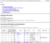
The following 2 tables show the first sample and its first 3 probes.
TargetID	CAF549.AVG_Beta	CAF549.Signal_A	CAF549.Signal_B	CAF549.Detection.Pval
cg00000292	0.303514376996805	5886	2565	3.68e-38
cg00002426	0.338360655737705	3027	1548	3.68e-38
cg00003994	0.0923276983094928	4886	497	3.68e-38
and
TargetID    08-132.AVG_Beta  08-132.Signal_A  08-132.Signal_B
cg00000029        0.6157420        2564.3650         4269.426
cg00000108        0.9355133         684.8924        11386.490
cg00000109        0.8333406         992.8285         5464.431
The software continues to ask the user whether he/she wishes to use the lumi package to normalize the data. If the user answers “Yes” to the question, data will be quantile color balance-adjusted, quantile normalized and then converted to the M values (log2 ratios of methylated over unmethylated normalized signal intensities) using functions in the lumi package, otherwise data will be converted to log2(beta/(1-beta)) values.
If the raw data file does not contain the signal intensities of methylated and unmethylated probes, or if the chip type is Golden Gate based, data will be read in using the methylumi package, and will be converted to log2(beta/(1-beta)) values. No matter what chip type it is, or whether normalization has been applied, the processed data will be treated equivalent to log2 ratio data.
For Illumina methylation data, there are 3 different options of annotation: 1) Annotate probes with the user’s own gene identifiers file; 2) SOURCE annotation and 3) Annotate probes with the annotation package available at Bioconductor. For options 1) and 2) the user is required to browse for their gene identifiers file, or specify the Gene identifier columns present alongside with the raw data file.
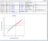
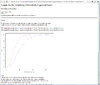
The first plot below shows the histogram of beta from one dataset. The second plot shows the relationship of beta vs M (M = log2(beta/(1-beta))).


In GEO, GSE19711 contains an ovarian cancer data on 540 whole blood samples (Illumina Infinium 27k Human DNA methylation Beadchip v1.2) and GSE42861 contains rheumatoid arthrotis data on 691 subjects (Illumina HumanMethylation450 BeadChip).
Analysis of 450k data using minfi by Jean-Philippe Fortin, Peter Hickey, Kasper Daniel Hansen and A cross-package Bioconductor workflow for analyzing methylation array data by Maksimovie, 2017.
llumina HumanMethylation450 BeadChip GPL13534 from GEO. For example, GSE38240 contains raw idat files (12x2).
Infinium MethylationEPIC data GPL21145 from GEO. For example GSE95531 contains raw idat files (8x2).
List of platforms from illumina and Homo sapiens where we can see the number of data rows, number of samples, number of series, and release dates. For example, 27k was released in 2009, 450k was released in 2011, EPIC was released in 2015.
RNA-Seq FPKM
ArrayTools -> Import Data -> Data Import Wizard -> RNA-Seq Data from Galaxy.
Format:
- http://cole-trapnell-lab.github.io/cufflinks/file_formats/#fpkm-tracking-format (multiple samples)
- http://www.broadinstitute.org/cancer/software/genepattern/file-formats-guide FPKM column format
- http://www.illumina.com/content/dam/illumina-marketing/documents/products/other/user-guide-rna-seq.pdf FPKM format. There are two kinds of fpkm files (genes and isoform). We care about genes only (genes.fpkm_tracking).
Some FPKM data:
- BRB-ArrayTools will take log2 transformation on the FPKM data and record the values in 'Filtered log intensity' worksheet.
- This human data was used in the paper: An integrative method to normalize RNA-Seq data. GSM1335718, GSM1335720, GSM1335722 to GSM1335756 (actually there are 37 samples). I combine the 4 samples and save it on here for testing importer in AT. The 'tracking_id' is Ensembl id and 'gene_short_name' is the gene symbol (for gene identifier dialog).
- http://www.ncbi.nlm.nih.gov/geo/query/acc.cgi?acc=GSE20846 No fpkm but the data is used by Trapnell 2012
For some reason, the genes.fpkm_tracking files downloaded from GEO is always one sample only. Ideally for multiple samples, the columns should have q0_FPKM, q0_FPKM_lo, q0_FPKM_hi, q0_status, q1_FPKM, q1_FPKM_lo, q1_FPKM_hi, q1_status, and so on as explained on here.
Because of the file format difference, we need to use the General Importer the RPKM data.
RNA-Seq raw count
ArrayTools -> Import Data -> RNA-Seq count data importer. If we choose the format of one text file, the whole flow is similar General Importer. However, the spot filter and normalization options will be grayed out in the 'Refilter, normalization and subset the data' dialog.
- In BRB-SeqTools, DESeq2 R package was used to import and normalize data. Normalized count data will be displayed in the “Filtered log intensity” worksheet. See <FilterAndNormalize.R>. The raw count values is saved in <BinaryData/RawData1> file.
junk <- DESeqDataSetFromMatrix(FilteredLog, colData=colData, design=~sampleName)
junk1 <- estimateSizeFactors(junk) # required for counts(, normalized=T)
# junk1 <- estimateDispersions(junk1) # NOT necessary from some examples
FilteredLog <- counts(junk1, normalized=T)
FilteredLog <- log2(FilteredLog+1)
- Normalized counts = counts / sizeFactor. See here for a numerical example.
- http://www.ncbi.nlm.nih.gov/geo/query/acc.cgi?acc=GSE45419 Breast cancer data. 32 samples. Raw count & fastq data are available. BioProject says the Project Type is Transcriptome or Gene expression. Samples are from 4 categories that can be identified from the first column in the 'Experiment descriptors' of the ArrayTools project.
Samples naming requirement
Several characters cannot be used in the samples names. These characters need to be removed from the header line of the expression table.
\ / : * ? < > | = +

A simple way to get rid of this issue is using R to convert these characters.
x <- read.delim("file.txt")
write.table(x, "newfile.txt", quote=F, row.names=F, sep="\t")
Annotation
SOURCE at standard
It requires the gene identifier contain one of Clone id, Accession number, Unigene cluster id, Entreze Gene ID or Gene symbol in order to search the SOURCE database.
when SOURCE at stanford is down
During the period of time when SOURCE website is down, our users will not be able to import annotations from SOURCE database. The bioconductor annotation packages will still work for users having Affymetrix or Illumina array data. For non-Affymetrix and non-Illumina chip users who are creating new projects, here are a couple of alternative solutions,
- If the user has an existing annotated project with an identical chip type to the project he/she is creating, he/she can import the annotations from the existing project. This can be done by clicking on 'ArrayTools -> Utilities -> Annotate the data -> Import annotations from an existing project';
- If the user has an annotation file available, during the process of importing, the user can choose to import annotations from this file. At the step of selecting Gene Identifiers, the user can browse for the Gene Identifiers file and check the option 'Annotate the project with these gene ids, instead of using the data from SOURCE database';
- If the user does not have an annotation file, for most commonly used commercial chips, the annotation files can be downloaded from GEO database at NCBI. For instance, the annotation file for the Agilent-014850 Whole Human Genome Microarray chip can be downloaded at http://www.ncbi.nlm.nih.gov/geo/query/acc.cgi?acc=GPL4133 by clicking on the 'Download full table' button. This downloaded annotation file can then be imported into BRB-ArrayTools following step 2).
Gene ST array annotation using aroma.affymetrix
The aroma.affymetrix can handle all single-channel Affymetrix chip types (they have a few multi-channel ones not supported), so my guess is that it is already supported. What's required for nearly all aroma analysis, is to have a CDF annotation file that defines the units and unit groups, e.g. probe sets of transcripts and exons, SNPs and so on. When Affymetrix is not providing a CDF, the challenge is to either find a custom CDF (e.g. BrainArray and GeneAnnot) or to create a one from the other types of annotation data they or Bioconductor provide, e.g. http://aroma-project.org/howtos.
(Update) aroma.affymetrix is replaced by oligo package to allow importing of Affymetrix gene 1.0, 1.1, 2.0 and 2.1 ST arrays in BRB-ArrayTools version 4.5.0.
Annotation with Bioconductor package - AnnotationDbi
The tool search gene symbol, accession number, UGCluster and Entrez ID columns. See <Annotations.bas>, <AnnotateGenes.bas> and MatchAffyAnnotation(), MatchBiocAnnotation() in <BiocUtil.R/> for the source code.
The AnnotationDbi package vignette used
library(xxx.db)
ls("package:xxx.db")
keytypes(xxx.db)

k=head(keys(xxx.db, keytype="PROBEID"))
select(xxx.db, keys=k, columns=c("SYMBOL", "GENENAME"), keytype="PROBEID")
And BRB-ArrayTools use mget() & get() in <BiocUtil.R>.
GO
- Pathway BiocViews
- http://www.bioconductor.org/packages/release/data/annotation/html/GO.db.html
- http://www.bioconductor.org/packages/release/data/annotation/html/hgu133plus2.db.html
AnnotationDbi: Introduction To Bioconductor Annotation Packages. Four methods are named: columns, keytypes, keys and select.
library(GO.db)
library(hgu133plus2)

class(GO.db)
# [1] "GODb"
# attr(,"package")
# [1] "AnnotationDbi"

keytypes(GO.db)
# [1] "DEFINITION" "GOID"       "ONTOLOGY"   "TERM"
keys(GO.db, keytype = "ONTOLOGY")
# [1] "BP"        "CC"        "MF"        "universal"
keys(GO.db, keytype = "GOID") %>% unique %>% length()
# [1] 45050

keytypes(hgu133plus2.db)
#  [1] "ACCNUM"       "ALIAS"        "ENSEMBL"      "ENSEMBLPROT"  "ENSEMBLTRANS"
#  [6] "ENTREZID"     "ENZYME"       "EVIDENCE"     "EVIDENCEALL"  "GENENAME"
# [11] "GO"           "GOALL"        "IPI"          "MAP"          "OMIM"
# [16] "ONTOLOGY"     "ONTOLOGYALL"  "PATH"         "PFAM"         "PMID"
# [21] "PROBEID"      "PROSITE"      "REFSEQ"       "SYMBOL"       "UCSCKG"
# [26] "UNIGENE"      "UNIPROT"
keys(hgu133plus2.db, keytype="GO") %>% unique %>% length()
# [1] 17983
KEGG
- Pathway BiocViews
- http://www.bioconductor.org/packages/release/data/annotation/html/KEGG.db.html
- https://www.biostars.org/p/14316/
BioCarta
- Pathway BiocViews
- www.biocarta.com
- https://cgap.nci.nih.gov/Pathways (BRB-ArrayTools used). See also DAVID Bioinformatics Resources website.
- https://www.bioconductor.org/packages/release/bioc/html/graphite.html
How many unique genes in KEGG/BioCarta
length(unique(unlist(lapply(pathway$kegg.keggrest.geneList, function(x) x$Symbol))))
# [1] 7878

length(unique(unlist(lapply(pathway$biocarta.geneList, function(x) x$Symbol))))
# [1] 1495
Genes with multiple ids (such as “NR_024445,BC041041,AK093927”)
Only the first id was used in gene annotation.
Gene symbol conversion problem from Excel
See Data science -> Gene name errors.
An Example of a Gene Annotation
Entrez ID/GeneID, Symbol, Name, Cytoband are more common.
| Entrez ID/GeneID | 6047 |
| Name | Ring finger protein 4 |
| Symbol GeneCards | RNF4 |
| Cytoband | 4p16.3 |
| GenBank Accession/RefSeq | NM_001185009 (Pomeroy, org.Hs.eg.db), AB000468 (Pomeroy, hu6800.db) |
| UniGene/UGCluster | Hs.740360 (BRCA) / Hs.66394 (Pomeroy) |
| CloneID | 50188 (BRCA) |
| GO | nucleus|TAS|GO:0005634//cellular component|nucleus|IEA|GO:0005634 |

Analysis
Normalization

Gene filtering

PERCENTAGE <- .20
LFC <- log2(1.5)
PERCENTILE <- .75

n <- ncol(x)  # genes x samples

# Minimum fold-change
tmp <- apply(x - apply(x, 1, median), 1, function(x) sum(x >= LFC | x <= (-1)*LFC))
tmpL1 <- tmp < ceiling(n * PERCENTAGE)       # to be excluded

# Log-ratio/log-intensity variation
tmp2 <- rowVars(x)
tmpL2 <- tmp2 <= quantile(tmp2, PERCENTILE)  # to be excluded

indg <- ! (tmpL1 | tmpL2)

x.filter <- x[indg, , drop=F]
An example from RNASeq where many of observations have a value zero. We will include this gene since this gene satisfies the minimum fold-change criterion.
x <- c(0, 0, 0, 0, 0, 0, 0, 0, 3.22, 0, 0, 0, 8.09, 0, 0.65, 0, 0,
0, 0, 0, 3.38, 0, 5.63, 7.46, 0, 0, 4.38, 0) # median(x) = 0
LFC = log2(1.5) = 0.58
sum(x >= LFC | x <= (-1)*LFC) = 7
ceiling(28 * PERCENTAGE) = ceiling(28 * .20) = 6

For the option of log-ratio variation by p-value: the filtering can be based on the variance for the gene across the arrays. One can exclude the x% of the genes with the smallest variances, where the percentile x is specified by the user. Or a statistical significance criterion based on the variance can be used. If the significance criterion is chosen, then the variance of the log-ratios for each gene is compared to the median of all the variances. Those genes not significantly more variable than the median gene are filtered out. The significance level threshold may be specified by the user. Specifically, the quantity [math]\displaystyle{ (n-1) Var_i / Var_{med} }[/math] is computed for each gene i. [math]\displaystyle{ Var_i }[/math] is the variance of the log intensity for gene i across the entire set of n arrays and [math]\displaystyle{ Var_{med} }[/math] is the median of these gene-specific variances. This quantity is compared to a percentile of the chi-square distribution with n-1 degrees of freedom. This is an approximate test of the hypothesis that gene i has the same variance as the median variance.
- [math]\displaystyle{ \begin{align} H_0: & \sigma^2=\sigma_0^2 \\ H_a: & \sigma^2 \gt \sigma_0^2 \end{align} }[/math]
Let [math]\displaystyle{ T = (N-1)(s/\sigma_0)^2 }[/math] and [math]\displaystyle{ s }[/math] is the sample standard deviation. Reject H0 if [math]\displaystyle{ T \gt χ^2_{1-\alpha, N-1} }[/math]. See Chi-Square Test for the Variance.
In the example, we accept/keep genes with p-value [math]\displaystyle{ \leq }[/math] threshold (on the dialog, it says genes are excluded if their p > threshold).
Random Variance Model
If RVM is checked, the model is estimated based on genes that are defined by Refilter, normalize, and subset the data dialog except some options are not applied (Utilities.base Line 2127)
- FoldDiffFilterValue (minimum fold-change in Gene filters)
- LogRatioFilterValue (log ratio variation in Gene filters)
- MinIntFilterValue (minimum intensity in Gene filters)
- GeneSubsetsFilterValue, GeneLabelsFilterValue, ProbeReductionFilterValue (in Gene subsets)
Note that the other 2 options (percent missing and percent absent) are still applied if they are checked.
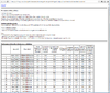
Below is a table of number of genes based on the default options in Refilter, normalize, and subset the data from 3 sample datasets included in BRB-ArrayTools.
| BRCA | Perou | Pomeroy | |
|---|---|---|---|
| Total | 3226 | 2998 | 7129 |
| RVM | 3226 | 2994 | 1958 |
| Filter | 2009 | 1902 | 1914 |
| Missing | No | Yes | No |
where
- Total: number of total genes in the project
- RVM: number of genes used in the RVM estimation
- Filter: number of filtered genes based on the 'Refilter, normalize, and subset the data'
- To view the genes used in RVM from the spreadsheet, we can turn off minimum fold-change option in the Gene filters tab/dialog. In other words, when we turn off minimum fold-change, the number of genes in RVM and Filter are the same (for example, 2994 genes for Perou and 1958 genes for Pomeroy).
- To view all genes from the spreadsheet, turn off all options in gene filters and gene subsets tabs. In other words, to make RVM to use all genes to do estimation, turn off all options in gene filters and gene subsets.
Function analysis using DAVID
See a tutorial from http://nihlibrary.ors.nih.gov/bioinfo/Microarray/Problem1.html
Best parameter or analysis to choose
Ask your local help desk.
For affy cel files, GCRMA has a memory problem and MAS5 is way too slow
It is a known problem for earlier versions of BRB-ArrayTools. The reason is statconnDCOM can only use 32-bit R. Since BRB-ArrayTools v4.3.0, a new engine 'Rserve' was adopted which can make use 64-bit R if the Windows OS is 64-bit. Therefore the memory issue for using GCRMA should be alleviated. (Update) The 64-bit OS still does not solve the memory problem; see a post and a workaround here from google forum.
BRB-ArrayTools uses justGCRMA() function in 'gcrma' package for GCRMA option and justMAS() function in 'simpleaffy' package for MAS5 option.
GO
- Gene annotation worksheet is used in Utilities -> Create genelist -> GO description.
- Bioconductor's GO package is used when we run gene set (gene ongology) class comparison.
- GO package was also used in the class comparison between groups of arrays -> Options -> Perform observed vs expected analyses. Only GO classes and parent classes with at least 5 observations in the selected subset and with an 'Observed vs. Expected' ratio of at least 2 (over-representation) are shown.
       | Sig genes      | not Sig gnes |
------------------------------------------
   GO  | obs=G^S        |              | g
       | exp=n*g/(g+ng) |              |
------------------------------------------
not GO |                |              | ng
------------------------------------------
       |    n           |              | g+ng
Broad MSigDB
Users will be guided to download the database. The following list shows the number of gene lists for human species. Note that the larger the number of gene lists, the longer it will take to get the HTML output.
- c1: Positional - 326
- c2: Curated - 3751
- c3: microRNA - 221 and TF - 615
- c4: Computed - 858
- c5: GO - 1454 (not included in the gene set analysis)
- C6: Oncogenic - 144
- c7: immunologic signature - 1888 (not included in the gene set analysis)
- H: hallmark - 50 (not included in the gene set analysis)
GSEA
In BRB-ArrayTools
- LS stands for log score. See Exploring gene expression data with class scores Pavlidis P, Lewis DP, Noble WS. 2002.
- LS statistic is also called Fisher's statistic. Gene-expression profiling identifies distinct subclasses of core binding factor acute myeloid leukemia Blood 2007.
- It was called Functional Class Score in Gene set analysis methods: statistical models and methodological differences 2014
- GSEA (class comparison -> gene set expression comparison): LS/KS permutation test finds gene sets which have more genes differentially expressed among the phenotype classes than expected by chance.
- The null hypothesis is the given gene set is a random selection from the project gene list. The alternative hypothesis is the gene set contains more genes differentially expressed between the classes being compared.
- Warning: Don't use the tool with a list of differentially expressed genes identified by class comparison analysis as the statistics are invalid.
- Re-sampling procedure was used, not permutation (so the procedure of computing the p-value is different from the permutation method Subramanian has used in 2005). The p-value is defined as the proportion of resampling selections for which the LS statistic is larger than the observed LS statistic.
- Default cutoff is p-value < .05.
- For survival data, LS/KS finds gene sets which have more genes differentially expressed with survival times than expected by chance.
- [math]\displaystyle{ LS = \sum_{i=1}^N (-\log p_i)/N }[/math]
- [math]\displaystyle{ KS = \max_{i=1}^N ( i/N - p_i), p_1 \leq p_2 \leq \cdots \leq p_N }[/math]
- GSA (class comparison -> gene set expression comparison): Efron-Tibshirani's test uses maxmean statistics to identify gene sets differentially expressed; gene scores in a gene set are unusually large. The scientific idea underlying enrichment, as nicely stated in Subramanian et al. (2005), is that a biologically related set of genes, perhaps representing a genetic pathway, could reveal its importance through a general effect on its constituent z-values, whether or not the individual zi’s were significantly non-zero.
- maxmean test statistic [math]\displaystyle{ S_{max} = \max \{\bar{s}^{(+)}, \bar{s}^{(-)} \}, s^{(+)} = \max(z, 0), s^{(-)} = -\min(z, 0) }[/math]
- The maxmean statisticis robust by design, not allowing a few large positive or negative gene score to dominate. See 16 of the paper. For example: suppose a gene set of 100 genes has scores [math]\displaystyle{ (-.5, -.5, \cdots, -.5, 10) }[/math]. Then [math]\displaystyle{ s^{(+)} = (0, 0, \cdots, 0, 10) }[/math] and [math]\displaystyle{ s^{(-)} = (-.5, -.5, \cdots, -.5, 0) }[/math]. So [math]\displaystyle{ \bar{s}^{(+)} = 10/100 = .1 }[/math] and [math]\displaystyle{ \bar{s}^{(-)} = 99*.5/100 = .495 }[/math]. Therefore [math]\displaystyle{ S_{max} = .495 }[/math].
- Maxmean is the mean of the positive or negative part of gene scores di in the gene set, whichever is large in absolute value. Specifically speaking, take all of the gene scores di in the gene set, and set all of the negative ones to zero. Then take the average of the positive scores, giving a positive part average avpos. Do the same for the negative side, setting the positive scores to zero, giving the negative part average avneg. Finally the score for the gene set is avpos if |avpos| > |avneg|, and otherwise it is avneg. Note that in this implementation, the positive or negative sign is relative to the first class. The meaning of the 1st and 2nd class is defined on the HTML output right above the table of significant gene sets. Efron and Tibshirani shows that this is often more powerful than the modified Kolmogorov-Smirnov statistic used in GSEA.
- The (+)/(-) signs in GSA test p-value column represent whether a gene set is positive or negative. A gene set is called positive if |avpos|>|avneg|. Therefore for example, if a gene set has a positive sign, then on average genes in arrays of 2nd class has larger expression values (after standardization) than in arrays in 1st class.
- Two different kinds of null distributions are consider: Randomization Model and Permutation Model.
- The randomization model tests the null hypothesis that the observed S is no bigger than what might be obtained by a random selection of S. Its defect concerns correlation between the genes.
- Permutation methods deal nicely with the correlation problem. The Permutation Model has a serious weakness of its own: it does not take into account the overall statistics (means, stdevs).
- For GSA, the authors combine the randomization and permutation ideas into a method that we call Restandardization.
- Over-represented pathway analysis (Utilities): Hypergeometric test finds Biocarta or KEGG pathways significantly enriched in the user's gene list (could be obtained other than the class comparison) for human or mouse species. Competitive null. The genes in the gene set do not have stronger association with the subject condition than other genes.
See also Statistics -> GSEA.
Over Representation Vs Enrichment Analysis and How informative are enrichment analyses really?
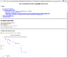
KEGG human diseases pathways color coding; Pathview
Utilities > Gene color coding for KEGG human disease pathways. The utility uses gene symbols to map the genes in the KEGG human disease pathways, and show the color coding of the intensities, ratios, or fold changes of the genes on the pathway diagrams. The imported data is a text file, and needs to have a Gene Symbol column, and an intensity/ratio/fold change column with tab delimited.
The input include:
- Disease
- One of the following options
- Select a sample name for log intensity/ratio values
- Select a class variable for log fold changes
- Import log intensity/ratio/fold change data
- Ouput file name (*.html)
Class prediction
Feature selection: Greedy pairs and SVM RFE
- Greedy pairs by Bo and Jonassen (Genome Biology 2002).
- The greedy-pairs approach first ranks all genes on the basis of individual t-score. Subsequently, this procedure first selects the best gene gi ranked by gene t-score, then finds the gene gj that together with gi, maximizes the pair t-score. These two genes are then removed from the gene set and the procedure is repeated on the remaining set until we have selected the desired number of genes. This approach is computationally much faster than all pairs, as only a subset of all gene pairs will be evaluated, but it may miss some pairs with high score.
- Details:
- consider gene 1 with the largest gene t-score, compute a1=(mean1-mean2)/var where var=(var1 + var2)/(n1+n2-2), var1 = sum(xi^2) - (sum xi)^2/n1.
- consider gene i, compute a2=(mean1-mean2)/var where var=(var1 + var2)/(n1+n2-2),
- create a virtual gene, xnew = a1*x[, gene1] + a2*x[, i]
- compute the T-statistic/pair t-score using the virtual gene. Find the gene gives the largest t-score. Done!
- repeat the process by excluding the 2 genes if npairs > 1.
- note: DLD axes a1 and a2 are similar but not the same as t-statistic. See formula (2) on the paper.
- R implementation Github
- In ArrayTools manual, it describes The procedure selects the best ranked gene gi and finds the one other gene gj that together with gi provides the best discrimination using as a measure the distance between centroids of the two classes with regard to the two genes when projected to the diagonal linear discriminant (DLS) axis.

- The Support Vector Machine Recursive Feature Elimination (SVM RFE) method uses an SVM classifier trained on the data to rank genes according to their contribution to the prediction performance. The SVM algorithm uses a weighted linear combination of the gene expressions as a discriminator between the two classes. This linear combination is selected to maximize the margin, or the distance between the worst classified samples and the discriminant plane.
Warning
Cross-validated error estimates for class prediction algorithms are invalid if the analysis is restricted to genes that are pre-selected to be differentially expressed between the classes. You are running class prediction on a subset of the genes but we cannot determine how you selected those genes. Proceed at your own risk. Do you wish to continue?
See Bias in CV error estimation
Compound covariate predictor
A Paradigm for Class Prediction Using Gene Expression Profiles
- [math]\displaystyle{ C_i = \sum_j t_j X_{ij} }[/math]
for gene [math]\displaystyle{ j }[/math] and sample [math]\displaystyle{ i }[/math]. A threshold is defined as [math]\displaystyle{ (C_1+C_2)/2 }[/math] where [math]\displaystyle{ C_1 }[/math] is the mean of [math]\displaystyle{ C_i }[/math] in class 1 and [math]\displaystyle{ C_2 }[/math] is the mean of [math]\displaystyle{ C_i }[/math] in class 2.
Bayesian compound covariate predictor
- [math]\displaystyle{ \begin{align} P(class 1|X) = \frac{P(X|class 1) * Prior(class 1)}{P(X|class 1)*Prior(class 1) + P(X | class 2)*Prior(class 2)} \end{align} }[/math]
where
- [math]\displaystyle{ \begin{align} P(X|class ~k) &\sim \textrm{dnorm}(\beta X, \mu_k, \sigma_{pooled}^2), k=1,2 \\ \beta &= \textrm{T} ~ \textrm{statistics} \\ \mu_k &= \textrm{mean} ~ \textrm{of} ~ \beta X_i ~ \textrm{for} ~ \textrm{data} ~ X_i ~ \textrm{in} ~ \textrm{class} ~ k \\ \sigma_{pooled}^2 &= \frac{\sum_i(X_i - \bar{X}^k)^2}{\sum_k (|C_k| -1)} \end{align} }[/math]
PAM
https://statweb.stanford.edu/~tibs/PAM/, Talk
Adaboost
Lasso logistic regression
Up to 6 clinical covariates.
Binary tree prediction for more than 2 classes
Random forests
Need to enter the number of genes randomly sampled as candidates at each split on each tree.
kNN and nearest centroid
train <- rbind(iris3[1:25,,1], iris3[1:25,,2], iris3[1:25,,3])
test <- rbind(iris3[26:50,,1], iris3[26:50,,2], iris3[26:50,,3])
cl <- factor(c(rep("s",25), rep("c",25), rep("v",25)))

library(class)
p1 <- knn(train, test, cl, k = 3, prob=TRUE)

library(WGCNA)
p2 = nearestCentroidPredictor(train, cl, test, simFnc = "dist") #?
p2$predictedTest

table(knn=p1, nc=p2$predictedTest)
#    nc
# knn  c  s  v
#   c 12  1 14
#   s  0 24  1
#   v  7  1 15
Below is a case NC is better than KNN (the new sample (green point) belongs to sensitive in reality).

Next is an example where 1NN is better than NC but it's b/c an outlier (the new sample (green point) is sensitive in reality).

Top scoring pairs
- Classifying gene expression profiles from pairwise mRNA comparisons Donald Geman et al 2004
- tspair package
- switchBox package
Quantitative trait analysis
Predict quantitative trait
algorithm (lars/lasso), include 2 way interaction (T/F), Training/predict samples indicators, % error threshold.
Survival analysis
Survival gene set analysis
Survival risk prediction
From the BRB-ArrayTools manual under the "Survival analysis" section:
- It is important to note that the risk group for each case was determined based on a predictor that did not use that case in any way in its construction. Hence, the (cross-validated) Kaplan-Meier curves are essentially unbiased and the separation between the curves gives a fair representation of the value of the expression profiles for predicting survival risk.
- (Model 1, gene expression only) The Survival Risk Group Prediction tool also provides an assessment of whether the association of expression data to survival data is statistically significant. A log-rank statistic is computed for the cross-validated Kaplan-Meier curves described above. Unfortunately, this log-rank statistic does not have the usual chi-squared distribution under the null hypothesis. This is because the data was used to create the risk groups. We can, however, obtain a valid statistical significance test by randomly shuffling the survival data among the cases and repeating the entire cross-validation process. ... The tail area of this null distribution beyond the value log-rank statistic LRd obtained for the real data is the permutation significance level for testing the null hypothesis that there is no relation between the expression data and survival.
- (Model 3, gene expression + clinical covariates) The Survival Risk Group Prediction tool also lets the user evaluate whether the expression data provides more accurate predictions than that provided by standard clinical or pathological covariates or a staging system. ... The cross-validated Kaplan-Meier curves and log-rank statistics are generated for those permutations and finally a p value is determined which measures whether the expression data adds significantly to risk prediction compared to the covariates.
Permutation method is used to test the following two hypotheses
- the genomic data is independent of survival data (Model 1)
- the genomic data do not add predictive accuracy to a survival risk model developed using a smaller number of standard covariates (Model 3)
R packages
- GCRMA: install cdf, probe, .db packages
- MAS5: install cdf, .db
Common download issue
Try to download/install manually in R console.
- lumi
source("http://bioconductor.org/biocLite.R")
biocLite("lumi", ask=F)
library(lumi)
- GO.db
source("http://bioconductor.org/biocLite.R")
biocLite("GO.db", ask=F)
- rtiff
install.packages('rtiff',repos='http://cran.r-project.org')
library('rtiff')
Some integrity check should be done. From my experience, R package installation often fails in VirtualBox environment where some library folder name becomes like file8b8182625c which is a temporary folder name. In my case the folder contains another sub-folder name call "RcppArmadillo" which is required by DESeq2 package. That is, even DESeq2 can be found under the library folder, some of its dependencies may be broken.
Recall that R package installation paths can be found by using the .libPaths() function.
Writable R package directory cannot be found
If you got the above message or saw the message C:/Program Files/R/R-X.Y.Z/lib is not writable, the possible causes/solutions are
- Another non-BRB-ArrayTools initialized R GUI/Terminal is running at the same time when BRB-ArrayTools is running.
- The current user does not have a full control on the C:\Program Files\R\ or a specific R version directory (even R was installed by the current user). Open the Windows Explorer, go to C:\Program Files\ , right click R folder and then choose Properties. In the 'Security' tab, click 'Edit' button. Check the box next to full control under User. Click OK button twice to enable the change. Done! After the change, the R's main packages will be still installed under the C:\Program Files\R\R-X.Y.Z\library folder. The other packages still go to Documents\R\win-library\X.Y\ directory if this folder has been created before; otherwise, new packages will go to C:\Program Files\R\R-X.Y.Z\library folder.

Download required R/Bioconductor (software) packages
Utilities -> Download/install required R/Bioconductor software packages. It runs the following R snippet.
ArrayToolsPath <-'C:/Program Files (x86)/ArrayTools'
source('C:/Program Files (x86)/ArrayTools/R/BiocUtil.r')
InstallAllRPackages()
Note: An error may happen and interrupt the installation. It is caused by updating the default R packages (e.g. cluster, codetools, foreign, lattice, Matrix, mgcv, nlme, survival) [R will pop up a message Would you like to use a personal library instead?]. It happened if the R packages were installed into C:\Users\USERNAME\Documents\R\win-library\x.y instead of C:\Program Files\R\R-x.y.z\library directory.

The same error can be reproduced by running the update.packages() function.
A simple way to fix the problem is to ensure the user has a full control on the folder C:\Program Files\R\R-X.Y.Z\library. See Writable R package directory cannot be found.
R
We have a report that R packages cannot be installed. If we answer 'yes' to the following question,
--------------
Question
--------------
Would you like to create a personal library
'C:\Users\<U+C591><U+C0C1><U+D654>\Documents/R/win-library/3.1' to install packages into?
we will get an error message:
  unable to create 'C:\Users\<U+C591><U+C0C1><U+D654>\Documents/R/win-library/3.1'.
In addition: Warning messages:
In dir.create(userdir, recursive = TRUE) :
  cannot create dir 'C:\Users\<U+C591><U+C0C1><U+D654>', reason 'Invalid argument'.
A similar report can be found on R help mailing list.
See also this and Wikipedia for Korean char.
Websites BRB-ArrayTools uses
List of websites and their purposes (No files were sent to a cloud to be processed)
http://linus.nci.nih.gov -- Check updates & registration
http://cran.r-project.org -- R packages
http://www.bioconductor.org -- Bioconductor packages & annotations
http://www.rforge.net -- R packages
http://r-forge.r-project.org -- R packages

http://software.broadinstitute.org/gsea -- BROAD
http://www.broad.mit.edu -- BROAD
http://source-search.princeton.edu -- Annotation
http://smd.stanford.edu -- Annotation
http://amigo.geneontology.org -- GO
http://cgap.nci.nih.gov -- Biocarta & KEGG
http://www.ncbi.nlm.nih.gov -- Gene symbols
http://nciarray.nci.nih.gov -- Gene symbols
http://www.godatabase.org -- GO
http://lymphochip.nih.gov -- Lymphoid malignancies
http://www.drugbank.ca -- Drug bank
http://brainarray.mbni.med.umich.edu -- Annotation
http://www.gene-regulation.com -- Transcription factor
http://microrna.sanger.ac.uk -- microRNA
http://www.mirbase.org -- microRNA
http://pfam.sanger.ac.uk --Protein domain
http://smart.embl.de -- Protein domain
http://cran.fhcrc.org -- R packages
http://java.com -- Java
http://dgidb.genome.wustl.edu -- Drug Gene Interaction database
http://www.genome.jp/kegg/pathway.html -- Human diseases pathways
http://www.genecards.org -- Gene information
Quirks
- Sometimes we got a weird error message. The trick is to shorten the project path.
> source.out <- try(source('C:/Program Files (x86)/ArrayTools/Excel/../plugins/DESeq2/DESeq.r')) > if (class(source.out)=='try-error') { cat(geterrmessage()); stop(); } Error in raw[, ind, drop = F] : object of type 'closure' is not subsettable - (This bug is fixed in v4.5.0 stable)
Do not place the project in a very deep path. Or you may get an error: reads "Error in 'exportToR' function" and then reads "Data was not successfully exported to R. Plug-in script is now aborting." - Do not include special characters (single/double quote, percent sign, etc), in the project name, output name, column header in the experiment descriptor worksheet. The special characters include * ? < > | = + ~ @ # $ % ^ & |. It is defined in <PublicFunctionProcedure.bas/CheckSpecialCharactersReturnBoolean>
- Do not sort the experiment descriptor worksheet.
- R's impute package tends to crash R when the number of genes is small.
- R's pamr package failed when the number of genes is only one. The error message is
Error in rep(1, p) : invalid 'times' argument
It is a bug in pamr.train() -> nsc(). - Write the R file used in plugins in a conventional format.
- Bioconductor package 'affxparser' does not work on Windows XP. The alternative is to use Affymetrix Expression Console to pre-process your ST arrays data and then import the .txt file that are outputted from Affymetrix Expression Console into ArrayTools by using the general format importer.
- Sometimes we need to delete the parameter file (under $ProjectFolder\BinaryData\DataParam) to solve a problem. For example, two projects were opened at the same time, or an analysis was broken during execution.
- Running in the VirtualBox environment can have some unexpected result. For example, running Import RNASeq count data wizard will hang EXCEL ("Not Responding" is showing on the title bar of the VB dialog. Also the CPU is busy too). If it is for testing purpose, we can subset the data and it will help.
- Some characters will be automatically changed by Excel. See below for some cases. To see a list of automatically converted symbols, sort the column. In additional to March, I see Sep and Dec. A solution to open the file without auto conversion is to change the column data format from 'General' to 'Text' in the import wizard. Also check HGNChelper R package.
excel real 1-Mar MARC1 2-Mar MARC2 1-Mar MARCH1 10-Mar MARCH10 2-Mar MARCH2
Run time errors
This is a collection of run-time errors from users' report or testing.
- error 1004: make sure the specified folder exists or file can be accessed.
- error 91: 'block variable not set'. It is rscproxy is not installed correctly. This should not happen again since rcom is no longer used.
- error 76: write permission, administrative privileges.
- error 75: write permission
- error 52. Bad file name or number
- error 53: Fie not found (RServeVBA.dll). Or the data is saved in a network drive (path starts with double backslash \\). Or there is a special symbol in the array file name. If the problem occurred when we launch Excel, try to install ArrayTools under C:\ instead of C:\Program Files (x86).
- error 14: Out of string space
- error 13: type mismatch. Special characters in files. Delete e.g. BinaryData\DataParam\ClassComparison.txt and run the class comparison again.
- error 9: subscription out of range. Variable name used in dialog is changed.
- error 7: out of memory
- error 6: Overflow. For example, when the input file is not tab delimited and we use RNA-Seq count data importer.
- error 5: invalid procedure call or argument.
- error '-2147319779' or '-2147221500': rscproxy package is not installed. This should not happen again since rcom is no longer used.
Large data
- If the number of arrays is small but the number of probesets is large (9 arrays and 947425 probesets), the random model estimation will have a problem (700,000 probesets limit).
*** Fortran program output is shown below ***
 Internal random seed = 123456789 will be used
 Global permutation tests will not be computed
 Univariate permutation tests will not be computed
 Randomized variance model will be used
forrtl: severe (157): Program Exception - access violation
- If the number of arrays is large and the number of probesets is large too (1248 arrays and 322695 probesets), we will get a clear error about insufficient memory:
*** Fortran program output is shown below ***
 Internal random seed = 123456789 will be used
 Global permutation tests will not be computed
 Univariate permutation tests will not be computed

forrtl: severe (41): insufficient virtual memory

Image              PC        Routine            Line        Source
ClassComparison.e  00479AF9  Unknown               Unknown  Unknown
Citing
Selected papers
- Acquired Initiating Mutations in Early Hematopoietic Cells of CLL Patients by Frederik Damm et al, 2014 AACR.
- Colorectal Cancer Classification and Survival Analysis Based on an Integrated RNA and DNA Molecular Signature, paper in Current Bioinformatics, 2020
Plugins Developers
- Experiment descriptor is a data frame with numerical or character data type (no factor). So we shall take extra care for cell with NA (numerical data type) or blank (character data type) value.
- Gene identifier is a data frame with factor data type.
Support
Self trouble-shooting
- If you got a message asking to send a bug report to [email protected], you can take a look at the <OutputReport.txt> file first (part of BugReport.tar.gz file).
- For example if the file shows Error : package 'pixmap' required by 'rtiff' could not be found, it indicates the rtiff R package cannot be found. While BRB-ArrayTools tries to install missing R packages automatically when it is running an analysis, the installation process can be broken by several reasons. In this case, you can close MS-Excel and all R processes and then open an R console and install pixmap package manually.
- Sometimes the R packages installation problem (e.g. Error in read.dcf(): cannot open the connection) can be solved by choosing a different mirror.
- Delete the ArrayTools folder (or only the Pathway folder if the problem comes from running the Biocarta Pathway analysis). Some extra old files will create an error even BRB-ArrayTools has been re-installed.
Send an email to [email protected]
Please provide enough information to us so we can understand the problem.
- If a bug report file was generated, be sure to send it to us.
- If the question is like 'what method or parameters should be choose to run my analysis', please consult other experienced people near you.
- Since the software depends on a couple factors like Windows operation system, MS-Office, R. Please provide us more detailed information about the software background including BRB-ArrayTools.
- When sending screenshots to us, please provide all error screenshots. If you only provide any random of them, it will create a misleading to us.
Check BRB-ArrayTools message board
https://secure.emmes.com/brbmessages/index.php
MISC
Illumina Genome Studio Manual
GEO
- Illumina. For example, the txt file <GSE13040_nonorm_nobkgd.txt> from GSE13040 (Illumina MouseRef-8 v2.0 expression beadchip) is close but not the one BRB-ArrayTools requires. We can modify the header to satisfy AT's requirement.
Affymetrix SNP arrays and cnt file for copy number analysis
To use the ‘Platform special importer’ for Affymetrix SNP arrays, the user should run the Copy Number Analysis Tool (CNAT) software, and output the *.CNT files in a batch process, where one *.CNT file is produced for each SNP array that was performed. The *.CNT output files should all be placed in one data folder, to be read by CGHTools. The “ProbeSet”, “Chromosome”, “Position” and “Log2Ratio” data columns will be automatically extracted from each *.CNT file.
See also goldenhelix.com for more about creating CNT files using the Affymetrix CNAT Batch Analysis Tool.
Affymetrix website contains some info about Chromosome Copy Number Analysis Tool (CNAT) software. This site provides links to command line tools to process 10K, 100K, and 500K (no SNP 5 or SNP 6) data from CHP file to CNT file. In fact, the tool download page here even provides sample output for download.
We may obtain raw files of copy number data from GEO website by searching 'affymetrix' and '10k' under 'Platforms' tab as keywords.
Another approach is to use the Copy Number Analyzer for Affymetrix GeneChip (CNAG) software and then process the data file to obtain data files in tab-delimited .txt format, which can be imported into BRB-CGHTools through the General Importer.
CGHTools
The CGHTools has several tools (segmentation, gain/loss, Gistic, pathway).
Once segmentation has been run, it is OK to jump to gain/loss, Gistic or pathway analysis. These 3 analyses have no mutual dependencies.
The CGHTools manual said when inferred integer copy number is imported at the importing step, the pathway enrichment analysis can be conducted without segmentation being performed.


We can find some Copy number data from GEO. For example, the GSE46452 has the Experiment type Genome variation profiling by genome tiling array while GSE26689 has an experiment type Genome variation profiling by array. GSE5013 from the paper has an experiment type Genome variation profiling by SNP array; SNP genotyping by SNP array. And GSE11960 has an experiment type Genome variation profiling by SNP array. GSE35873 has a type Genome variation profiling by SNP array; Genome binding/occupancy profiling by SNP array.
Copy number variation and gene expression are related in Identification of genes with a correlation between copy number and expression in gastric cancer where CGH data is in GSE33428 and gene expression data is in GSE33335. Another study is in GSE10744.
Some tutorial created by Sean Davis.