File:KMannotation.png
Jump to navigation
Jump to search
No higher resolution available.
KMannotation.png (732 × 546 pixels, file size: 58 KB, MIME type: image/png)
Summary
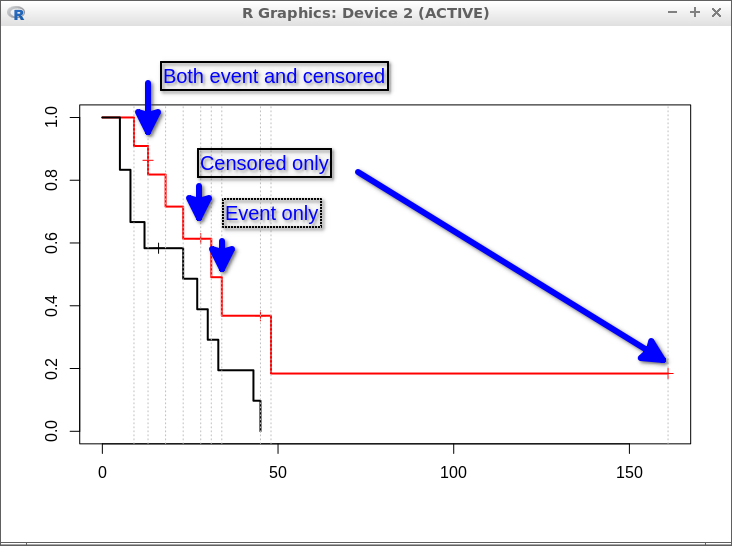
library(survival)
sf <- survfit(Surv(time, status) ~ x, data = aml)
plot(sf, col=c('red', 'black'))

rbind(time=aml$time[aml$x == 'Maintained'], status=aml$status[aml$x == 'Maintained'])
#        [,1] [,2] [,3] [,4] [,5] [,6] [,7] [,8] [,9] [,10] [,11]
# time      9   13   13   18   23   28   31   34   45    48   161
# status    1    1    0    1    1    0    1    1    0     1     0

unique(aml$time[aml$x == 'Maintained'])
#  [1]   9  13  18  23  28  31  34  45  48 161

summary(sf)
# Call: survfit(formula = Surv(time, status) ~ x, data = aml)
#
#                 x=Maintained
#  time n.risk n.event survival std.err lower 95% CI upper 95% CI
#     9     11       1    0.909  0.0867       0.7541        1.000
#    13     10       1    0.818  0.1163       0.6192        1.000
#    18      8       1    0.716  0.1397       0.4884        1.000
#    23      7       1    0.614  0.1526       0.3769        0.999
#    31      5       1    0.491  0.1642       0.2549        0.946
#    34      4       1    0.368  0.1627       0.1549        0.875
#    48      2       1    0.184  0.1535       0.0359        0.944
#
#                 x=Nonmaintained
#  time n.risk n.event survival std.err lower 95% CI upper 95% CI
#     5     12       2   0.8333  0.1076       0.6470        1.000
#     8     10       2   0.6667  0.1361       0.4468        0.995
#    12      8       1   0.5833  0.1423       0.3616        0.941
#    23      6       1   0.4861  0.1481       0.2675        0.883
#    27      5       1   0.3889  0.1470       0.1854        0.816
#    30      4       1   0.2917  0.1387       0.1148        0.741
#    33      3       1   0.1944  0.1219       0.0569        0.664
#    43      2       1   0.0972  0.0919       0.0153        0.620
#    45      1       1   0.0000     NaN           NA           NA
The plot is annotated using ksnip.
Case 2: no median survival time. Smallest survival time > .5.
aml2 <- aml; aml2[24:46, 'time'] <- 161; aml2[24:46, 'status'] <- 0
plot(survfit(Surv(time, status) ~ 1, aml2))
summary(survfit(Surv(time, status) ~ 1, aml2))

# Call: survfit(formula = Surv(time, status) ~ 1, data = aml2)
#
#  time n.risk n.event survival std.err lower 95% CI upper 95% CI
#     5     46       2    0.957  0.0301        0.899        1.000
#     8     44       2    0.913  0.0415        0.835        0.998
#     9     42       1    0.891  0.0459        0.806        0.986
#    12     41       1    0.870  0.0497        0.777        0.973
#    13     40       1    0.848  0.0530        0.750        0.958
#    18     37       1    0.825  0.0563        0.722        0.943
#    23     36       2    0.779  0.0618        0.667        0.910
#    27     34       1    0.756  0.0641        0.640        0.893
#    30     32       1    0.733  0.0663        0.614        0.875
#    31     31       1    0.709  0.0682        0.587        0.856
#    33     30       1    0.685  0.0699        0.561        0.837
#    34     29       1    0.662  0.0714        0.536        0.817
#    43     28       1    0.638  0.0726        0.510        0.798
#    45     27       1    0.614  0.0737        0.486        0.777
#    48     25       1    0.590  0.0747        0.460        0.756
Case 3: Still no median survival time. One event at the largest survival time (vertical bar goes down a little bit).
aml2[46, 'status'] <- 1
plot(survfit(Surv(time, status) ~ 1, aml2))
summary(survfit(Surv(time, status) ~ 1, aml2))
# Call: survfit(formula = Surv(time, status) ~ 1, data = aml2)
#
#  time n.risk n.event survival std.err lower 95% CI upper 95% CI
#     5     46       2    0.957  0.0301        0.899        1.000
#     8     44       2    0.913  0.0415        0.835        0.998
#     9     42       1    0.891  0.0459        0.806        0.986
#    12     41       1    0.870  0.0497        0.777        0.973
#    13     40       1    0.848  0.0530        0.750        0.958
#    18     37       1    0.825  0.0563        0.722        0.943
#    23     36       2    0.779  0.0618        0.667        0.910
#    27     34       1    0.756  0.0641        0.640        0.893
#    30     32       1    0.733  0.0663        0.614        0.875
#    31     31       1    0.709  0.0682        0.587        0.856
#    33     30       1    0.685  0.0699        0.561        0.837
#    34     29       1    0.662  0.0714        0.536        0.817
#    43     28       1    0.638  0.0726        0.510        0.798
#    45     27       1    0.614  0.0737        0.486        0.777
#    48     25       1    0.590  0.0747        0.460        0.756
#   161     24       1    0.565  0.0756        0.435        0.735
Case 4: With median survival time (last survival < .5). Lots of events at the largest survival time (vertical bar goes down a lot).
aml2 <- aml; aml2[24:46, 'time'] <- 161; aml2[24:46, 'status'] <- 1
plot(survfit(Surv(time, status) ~ 1, aml2))
summary(survfit(Surv(time, status) ~ 1, aml2))
# Call: survfit(formula = Surv(time, status) ~ 1, data = aml2)
#
#  time n.risk n.event survival std.err lower 95% CI upper 95% CI
#     5     46       2   0.9565  0.0301      0.89937        1.000
#     8     44       2   0.9130  0.0415      0.83514        0.998
#     9     42       1   0.8913  0.0459      0.80575        0.986
#    12     41       1   0.8696  0.0497      0.77749        0.973
#    13     40       1   0.8478  0.0530      0.75013        0.958
#    18     37       1   0.8249  0.0563      0.72168        0.943
#    23     36       2   0.7791  0.0618      0.66695        0.910
#    27     34       1   0.7562  0.0641      0.64048        0.893
#    30     32       1   0.7325  0.0663      0.61350        0.875
#    31     31       1   0.7089  0.0682      0.58705        0.856
#    33     30       1   0.6853  0.0699      0.56107        0.837
#    34     29       1   0.6616  0.0714      0.53553        0.817
#    43     28       1   0.6380  0.0726      0.51040        0.798
#    45     27       1   0.6144  0.0737      0.48566        0.777
#    48     25       1   0.5898  0.0747      0.46010        0.756
#   161     24      23   0.0246  0.0243      0.00355        0.170
File history
Click on a date/time to view the file as it appeared at that time.
| Date/Time | Thumbnail | Dimensions | User | Comment | |
|---|---|---|---|---|---|
| current | 16:59, 3 May 2020 | | 732 × 546 (58 KB) | Brb (talk | contribs) | Reverted to version as of 16:57, 3 May 2020 (EDT) |
| 16:58, 3 May 2020 |  | 732 × 546 (47 KB) | Brb (talk | contribs) | Reverted to version as of 21:54, 2 May 2020 (EDT) | |
| 16:57, 3 May 2020 |  | 732 × 546 (58 KB) | Brb (talk | contribs) | ||
| 21:54, 2 May 2020 |  | 732 × 546 (47 KB) | Brb (talk | contribs) | <pre> library(survival) sf <- survfit(Surv(time, status) ~ x, data = aml) plot(sf, col=c('red', 'black')) </pre> |
You cannot overwrite this file.
File usage
There are no pages that use this file.