GSEA: Difference between revisions
(→MSigDB) |
|||
| Line 443: | Line 443: | ||
https://www.gsea-msigdb.org/gsea/msigdb/ | https://www.gsea-msigdb.org/gsea/msigdb/ | ||
* C1: Hallmark | * C1: Hallmark | ||
* C2: Curated gene sets including BioCarta | * C2: Curated gene sets including BioCarta, KEGG, Reactome | ||
* C5: Oncology | * C5: Oncology | ||
Revision as of 11:08, 30 June 2022
Basic
https://en.wikipedia.org/wiki/Gene_set_enrichment_analysis
Determines whether an a priori defined set of genes shows statistically significant, concordant differences between two biological states
- https://www.bioconductor.org/help/course-materials/2015/SeattleApr2015/E_GeneSetEnrichment.html, https://www.bioconductor.org/help/course-materials/2009/SeattleApr09/gsea/HyperG_Lecture.pdf. For hypergeometric test, it is
- finding Biocarta or KEGG pathways significantly enriched in the user's gene list
- Are DE genes in the set more common than DE genes not in the set?.
- Are selected genes more often in the GO category than expected by chance? (one-tailed)
We can draw a 2x2 table or a venn diagram to see the diagram.
In gene set Yes No DE Yes No
- Gene List Enrichment Analysis dhyper(), binom.test(), fisher.test().
- Pathway Commons
- Gene set analysis methods: statistical models and methodological differences 2014
- http://software.broadinstitute.org/gsea/index.jsp, Subramanian, et al 2005 paper
- HOW TO PERFORM GSEA - A tutorial on gene set enrichment analysis for RNA-seq (video)
- Algorithm. GSEA walks down the ranked list of genes, increasing a running-sum statistic when a gene belongs to the set and decreasing it when the gene does not.
- Interpretation of 3 enrichment plots. The 1st plot (ES on y-axis) tells you how over or under expressed is your gene respect to the ranked list. The 2nd part of the graph (barcode-like) shows where the members of the gene set appear in the ranked list of genes. The 3rd graph (y=ranked list metric, x=rank) shows how your metric is distributed along the list.
- slides with formulas.
- What does a negative enrichment score mean? A negative NES will indicate that the genes in the set S will be mostly at the bottom of your list L.
- GSEA R Implementation from GSEA-MSigDB.
- READMe.
- Using GSEA.1.0.R
- Statistical power of gene-set enrichment analysis is a function of gene set correlation structure by SWANSON 2017
- Towards a gold standard for benchmarking gene set enrichment analysis, GSEABenchmarkeR package
- piano package
- clusterProfiler package and the online book.
- Gene-set Enrichment with Regularized Regression Fang 2019
- msigdbr package. MSigDB Gene Sets for Multiple Organisms in a Tidy Data Format.
- Best method/package for Gene Set Enrichment Analysis in R? and the gage package
- ES could be negative; see Genome 559: Introduction to Statistical and Computational Genomics
- multiGSEA: a GSEA-based pathway enrichment analysis for multi-omics data
- How to use DAVID for functional annotation of genes, Using DAVID for Functional Enrichment Analysis in a Set of Genes (Part 1), (Part 2) (video)
Two categories of GSEA procedures:
- Competitive: compare genes in the test set relative to all other genes.
- Self-contained: whether the gene-set is more DE than one were to expect under the null of no association between two phenotype conditions (without reference to other genes in the genome). For example the method by Jiang & Gentleman Bioinformatics 2007
See also BRB-ArrayTools -> GSEA.
Interpretation
- XXX class is associated with the XXX gene sets (GSVA vignette)
- XXX subtype is characterized by the expression of XXX markers, thus we expect it to correlate with the XXX gene set (GSVA vignette)
- The XXX subtype shows high expression of XXX genes, thus the XXX gene sets is highly enriched for this group (GSVA vignette)
Calculation
FDR cutoff
Why does GSEA use a false discovery rate (FDR) of 0.25 rather than the more classic 0.05?
edgeR
Over-representation analysis. ?goana and ?kegga. See UserGuide 2.14 Gene ontology (GO) and pathway analysis.
fgsea
fgsea package and download stat
- ?exampleRanks gives a hint about how it was obtained. It is actually the t-statistic, not logFC.
... fit2 <- eBayes(fit2) de <- data.table(topTable(fit2, adjust.method="BH", number=12000, sort.by = "B"), keep.rownames = TRUE) colnames(de) plot(de$t, exampleRanks[match(de$rn, names(exampleRanks))]) # 45 degrees straight line range(de$t) # [1] -62.22877 52.59930 range(exampleRanks) # [1] -63.33703 53.28400 range(de$logFC) # [1] -11.56067 12.57562 - vignette
library(fgsea)
library(ggplot2)
data(examplePathways) # a list of length 1457 (pathways)
data(exampleRanks)    # a vector of length 12000 (genes)
set.seed(42)
fgseaRes <- fgsea(pathways = examplePathways,
                   stats    = exampleRanks,
                   minSize  = 4,
                   maxSize  =10) # choose a small gene set in order to see the detail

head(fgseaRes[order(pval), ], 1)
#                            pathway         pval         padj   log2err        ES
# 1: 5991601_Phosphorylation_of_Emi1 2.461461e-07 9.501241e-05 0.6749629 0.9472236
#         NES size                           leadingEdge
# 1: 2.082967    6 107995,12534,18817,67141,268697,56371

plotEnrichment(examplePathways[["5991601_Phosphorylation_of_Emi1"]], exampleRanks)
# still hard to understand the graph

# Reduce the total number of genes
match(examplePathways[["5991601_Phosphorylation_of_Emi1"]], names(exampleRanks))
# [1] 11678 11593 11362 11553 11953 11383    NA    NA
i <- match(examplePathways[["5991601_Phosphorylation_of_Emi1"]], names(exampleRanks))
i <- na.omit(i)
# plotEnrichment(examplePathways[["5991601_Phosphorylation_of_Emi1"]], exampleRanks[i])
# GSEA statistic is not defined when all genes are selected
plotEnrichment(examplePathways[["5991601_Phosphorylation_of_Emi1"]], exampleRanks[c(1,i)])
# Easy to understand
exampleRanks[c(1,i)]
#    170942     12534     18817     56371     67141    107995    268697
# -63.33703  15.16265  13.46935  10.46504  12.70504  28.36914  10.67534
Note shifting exampleRanks values will change the enrichment scores
plotEnrichment(examplePathways[[1]],
                exampleRanks) + labs(title="Programmed Cell Death")
            # like sin() with one period
range(exampleRanks)
# [1] -63.33703  53.28400
plotEnrichment(examplePathways[[1]],
                exampleRanks+64) + labs(title="Programmed Cell Death")
            # like a time series plot
plotEnrichment(examplePathways[[1]],
                exampleRanks-54) + labs(title="Programmed Cell Death")
            # same problem if we shift exampleRanks to all negative
including NE, NES, pval, etc. So it is not rank-based.
set.seed(42)
fgseaRes2 <- fgsea(pathways = examplePathways,
                   stats    = exampleRanks+2, # OR 2*(exampleRanks+2)
                   minSize  = 4,
                   maxSize  =10)
identical(fgseaRes, fgseaRes2)
# [1] FALSE
R> fgseaRes[1:3, c("ES", "NES", "pval")]
           ES        NES      pval
1: -0.3087414 -0.6545067 0.8630705
2:  0.4209054  1.0360288 0.4312268
3: -0.4065043 -0.8617561 0.6431535
R> fgseaRes2[1:3, c("ES", "NES", "pval")]
           ES        NES      pval
1:  0.4554877  0.8284722 0.7201767
2:  0.5520914  1.1604366 0.2833333
3: -0.2908641 -0.5971951 0.9442724
However, scaling won't change anything.
set.seed(42) fgseaRes3 <- fgsea(pathways = examplePathways, stats = 2*exampleRanks, minSize = 4, maxSize =10) identical(fgseaRes, fgseaRes3) # [1] TRUE - ?collapsePathways. Collapse list of enriched pathways to independent ones.
- DESeq results to pathways in 60 Seconds with the fgsea package
- Performing GSEA using MSigDB gene sets in R
Subramanian algorithm
In the plot, (x-axis) genes are sorted by their expression across all samples. Y-axis represents enrichment score. See HOW TO PERFORM GSEA - A tutorial on gene set enrichment analysis for RNA-seq. Bars represents genes being in the gene set. Genes on the LHS/RHS are more highly expressed in the experimental/control group. Small p means this gene set is enriched in this experimental sample.
Rafael A Irizarry
Gene set enrichment analysis made simple
multiGSEA
multiGSEA - Combining GSEA-based pathway enrichment with multi omics data integration.
Plot
- Chapter 12 Visualization of Functional Enrichment Result, enrichplot::gseaplot() or enrichplot::gseaplot2() from Bioconductor
- GSEA 从数据到美图 where step4output.Rdata is available on github. Some quirks:
# geneset$term = str_remove(geneset$term,"HALLMARK_")
- Plot rank densities from singscore::plotRankDensity() from Bioc
- fgsea::plotGseaTable() from Bioc
- Interpreting this plot from GSEA
Single sample
singscore
- singscore
- Paper Single sample scoring of molecular phenotypes. Our approach does not depend upon background samples and scores are thus stable regardless of the composition and number of samples being scored. In contrast, scores obtained by GSVA, z-score, PLAGE and ssGSEA can be unstable when less data are available (NS < 25). Simulation was conducted.
- SingscoreAMLMutations
- TotalScore = UpScore + DownScore
- centerScore and knownDirection parameters used in generateNull() and simpleScore() functions.
- On the paper, epithelial and mesenchymal gene sets are up-regulated and TGFβ-EMT signature is bidirectional.
- The pvalue calculation seems wrong. For example, the first sample D_Ctrl_R1 returns p=0.996 but it should be 2*(1-.996) according to the null distribution plot. However, the 1st sample is a control sample so we don't expect it has a large score; its p-value should be large?
- Gene-set enrichment analysis workshop. Also use ExperimentHub, SummarizedExperiment, emtdata, GSEABase, msigdb, edgeR, limma, vissE, igraph & patchwork packages.
- Functions in the GSEABase package help with reading, parsing and processing the signatures.
ssGSEA
- https://github.com/broadinstitute/ssGSEA2.0
- ssGSEAProjection (v9.1.2). Each ssGSEA enrichment score represents the degree to which the genes in a particular gene set are coordinately up- or down-regulated within a sample.
- single sample GSEA (ssGSEA) from http://baderlab.org/
- How single sample GSEA works
- Data formats gct (expression data format), gmt (gene set database format).
- gmt file can be read by GSA.read.gmt()
- gmt file can be read by clusterProfiler::read.gmt(). See R做GSEA富集分析
- ssGSEA produced by Broad Gene Pattern is different from one produced by gsva package.
- Actually they are not compatible. See a plot in singscore paper.
- Gene Pattern also compute p-values testing the Spearman correlation
- GSVA and SSGSEA for RNA-Seq TPM data.
- Generally, negative enrichment values imply down-regulation of a signature / pathway; whereas, positive values imply up-regulation.
- The idea is to then conduct a differential signature / pathway analysis (using, for example, limma) so that you can have, in addition to differentially expressed genes, differentially expressed signatures / pathways.
- GSVA vignette. In GSEA Subramanian et al. (2005) it is also observed that the empirical null distribution obtained by permuting phenotypes is bimodal and, for this reason, significance is determined independently using the positive and negative sides of the null distribution.
- Tips:
- Pre-processing RNA-seq data (normalization and transformation) for GSVA
- pre-filtering gene sets for GSVA/ssGSEA
- kcdf parameter it is only relevant when method="gsva". See Method and kcdf arguments in gsva package and debugging source code.
- mx.diff: Offers two approaches to calculate the enrichment statistic (ES) from the KS random walk statistic. mx.diff=FALSE: ES is calculated as the maximum distance of the random walk from 0. mx.diff=TRUE (default): ES is calculated as the magnitude difference between the largest positive and negative random walk deviations.
- min.sz=1, max.sz=Inf
- 纯R代码实现ssGSEA算法评估肿瘤免疫浸润程度. The pheatmap package was used to draw the heatmap. Original paper.
- fpkm expression data was sorted by gene name & median values. Duplicated genes are removed. The data is transformed by log2(x+1) before sent to gsva()
- NES scores are scaled and truncated to [-2, 2]. The scores are further scaled to have the range [0,1] before sending it to the heatmap function
- gsva() from the GSVA package has an option to compute ssGSEA. 单样本基因集富集分析 --- ssGSEA (it includes the formula from Barbie's paper). The output of gsva() is a matrix of ES (# gene sets x # samples). It does not produce plots nor running the permutation tests. Notice the option ssgsea.norm. Note ssgsea.norm = TRUE (default) option will scale ES by the absolute difference of the max and min ES; Unscaled ES / (max(unscaled ES) - min(unscaled ES)). So the scaled ES values depends on the included samples. But it seems the impact of the included samples is small from some real data. See the source code on github and on how to debug an S4 function.
library(GSVA) library(heatmaply) p <- 10 ## number of genes n <- 30 ## number of samples nGrp1 <- 15 ## number of samples in group 1 nGrp2 <- n - nGrp1 ## number of samples in group 2 ## consider three disjoint gene sets geneSets <- list(set1=paste("g", 1:3, sep=""), set2=paste("g", 4:6, sep=""), set3=paste("g", 7:10, sep="")) ## sample data from a normal distribution with mean 0 and st.dev. 1 set.seed(1234) y <- matrix(rnorm(n*p), nrow=p, ncol=n, dimnames=list(paste("g", 1:p, sep="") , paste("s", 1:n, sep=""))) ## genes in set1 are expressed at higher levels in the last 'nGrp1+1' to 'n' samples y[geneSets$set1, (nGrp1+1):n] <- y[geneSets$set1, (nGrp1+1):n] + 2 gsva_es <- gsva(y, geneSets, method="ssgsea") dim(gsva_es) # 3 x 30 hist(gsva_es) # bi-modal range(gsva_es) # [1] -0.4390651 0.5609349 ## build design matrix design <- cbind(sampleGroup1=1, sampleGroup2vs1=c(rep(0, nGrp1), rep(1, nGrp2))) ## fit the same linear model now to the GSVA enrichment scores fit <- lmFit(gsva_es, design) ## estimate moderated t-statistics fit <- eBayes(fit) ## set1 is differentially expressed topTable(fit, coef="sampleGroup2vs1") # logFC AveExpr t P.Value adj.P.Val B # set1 0.5045008 0.272674410 8.065096 4.493289e-12 1.347987e-11 17.067380 # set2 -0.1474396 0.029578749 -2.315576 2.301957e-02 3.452935e-02 -4.461466 # set3 -0.1266808 0.001380826 -2.060323 4.246231e-02 4.246231e-02 -4.992049 heatmaply(gsva_es) # easy to see a pattern # samples' clusters are not perfect heatmaply(gsva_es, scale = "none") # 'scale' is not working? heatmaply(y, Colv = F, Rowv= F, scale = "none") # not easy to see a pattern - If we set ssgsea.norm=FALSE, do we get the same results when we compute ssgsea using a subset of samples?
gsva1 <- gsva(y, geneSets, method="ssgsea", ssgsea.norm = FALSE)
gsva2 <- gsva(y[, 1:2], geneSets, method="ssgsea", ssgsea.norm = FALSE)
range(abs(gsva1[, 1:2] - gsva2)) # [1] 0 0
- Verify ssgsea.norm = TRUE option.
gsva_es <- gsva(y, geneSets, method="ssgsea")
gsva1 <- gsva(y, geneSets, method="ssgsea", ssgsea.norm = FALSE)
gsva2 <- gsva1 / abs(max(gsva1) - min(gsva1)) # abs(max(gsva1) - min(gsva1)) 8.9

range(gsva_es)              # [1] -0.4390651  0.5609349
range(abs(gsva_es - gsva2)) # [1] 0 0
- Only ranks matters! If I replace the sample 1 gene expression values with the ranks, the ssgsea scores are not changed at all.
y2 <- y
y2[, 1] <- rank(y2[, 1])
gsva2 <- gsva(y2, geneSets, method="ssgsea")
gsva_es[, 1]
#      set1       set2       set3
# 0.1927056  0.1699799 -0.1782934
gsva2[, 1]
#      set1       set2       set3
# 0.1927056  0.1699799 -0.1782934
all.equal(gsva_es, gsva2)
# [1] TRUE

# How about the reverse ranking? No that will change everything.
# The one with the smallest value was assigned one according to
# the definition of 'rank'
y3[, 1] <- 11 - y2[, 1]
gsva3 <- gsva(y3, geneSets, method="ssgsea")
gsva3[, 1]
#        set1         set2         set3
#-0.054991319 -0.009603802  0.191733634

cbind(y[, 1], y2[, 1], y3[, 1])
#           [,1] [,2] [,3]
# g1  -1.2070657    2    9
# g2   0.2774292    7    4
# g3   1.0844412   10    1
# g4  -2.3456977    1   10
# g5   0.4291247    8    3
# g6   0.5060559    9    2
# g7  -0.5747400    4    7
# g8  -0.5466319    6    5
# g9  -0.5644520    5    6
# g10 -0.8900378    3    8
- Is mx.diff useful? No.
gsva4 <- gsva(y, geneSets, method="ssgsea", mx.diff = FALSE)
all.equal(gsva_es, gsva4)
# [1] TRUE
- A simple implementation of ssGSEA (single sample gene set enrichment analysis)
- Use "ssgsea-gui.R". The first question is a folder containing input files GCT. The 2nd question is about gene set database in GMT format. This has to be very restrict. For example, "ptm.sig.db.all.uniprot.human.v1.9.0.gmt" and "ptm.sig.db.all.sitegrpid.human.v1.9.0.gmt" provided in github won't work with the example GCT file.
setwd("~/github/ssGSEA2.0/")
source("ssgsea-gui.R")
# select a folder containing gct files; e.g. PI3K_pert_logP_n2x23936.gct
# select a gene set file; e.g. <ptm.sig.db.all.flanking.human.v1.8.1.gmt>
A new folder (e.g. 2021-03-01) will be created under the same parent folder as the gct file folder.
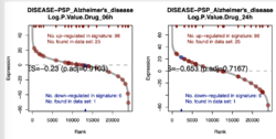
tree -L 1 ~/github/ssGSEA2.0/example/gct/2021-03-20/

├── PI3K_pert_logP_n2x23936_ssGSEA-combined.gct
├── PI3K_pert_logP_n2x23936_ssGSEA-fdr-pvalues.gct
├── PI3K_pert_logP_n2x23936_ssGSEA-pvalues.gct
├── PI3K_pert_logP_n2x23936_ssGSEA-scores.gct
├── PI3K_pert_logP_n2x23936_ssGSEA.RData
├── parameters.txt
├── rank-plots
├── run.log
└── signature_gct

tree ~/github/ssGSEA2.0/example/gct/2021-03-20/rank-plots | head -3
# 102 files. One file per matched gene set
├── DISEASE.PSP_Alzheime_2.pdf
├── DISEASE.PSP_breast_c_2.pdf

tree ~/github/ssGSEA2.0/example/gct/2021-03-20/signature_gct | head -3
# 102 files. One file per matched gene set
├── DISEASE.PSP_Alzheimer.s_disease_n2x23.gct
├── DISEASE.PSP_breast_cancer_n2x14.gct
Since the GCT file contains 2 samples (the last 2 columns), ssGSEA produces one rank plot for each gene set (with adjusted p-value & the plot could contain multiple samples). The ES scores are saved in <PI3K_pert_logP_n2x23936_ssGSEA-scores> and adjust p-values are saved in <PI3K_pert_logP_n2x23936_ssGSEA-fdr-pvalues>.
- Some possible problems using ssGSEA to replace GSEA for DE analysis? See a toy example on Single Sample GSEA (ssGSEA) and dynamic range of expression. PS: the rank values table is wrong; they should be reversed.
- In general terms, PLAGE and z-score are parametric and should perform well with close-to-Gaussian expression profiles, and ssGSEA and GSVA are non-parametric and more robust to departures of Gaussianity in gene expression data. See Method and kcdf arguments in gsva package
- Some discussions from biostars.org. Find -> "ssgsea"
- Some papers.
- 【生信分析 3】教你看懂GSEA和ssGSEA分析结果. No groups/classes in the data (6:33). Output is a heatmap. Each value is computed sample by sample. Rows = gene set. Columns = (sorted by the 1st gene set) samples.

escape
escape - Easy single cell analysis platform for enrichment. Github.
Benchmark
Toward a gold standard for benchmarking gene set enrichment analysis Geistlinger, 2021. GSEABenchmarkeR package in Bioconductor.
phantasus
- phantasus Visual and interactive gene expression analysis. read.gct(), write.gct(), getGSE(), loadGEO(), gseaPlot().
- Using Phantasus application
Selected papers
- On the influence of several factors on pathway enrichment analysis Mubeen 2022
- Popularity and performance of bioinformatics software: the case of gene set analysis Xie 2021
- Gene set analysis approaches for RNA-seq data: performance evaluation and application guideline Rahmatallah 2015. Simulated RNA-Seq data was considered too.
- Gene set analysis methods: a systematic comparison Mathur, 2018
- A Comparison of Gene Set Analysis Methods in Terms of Sensitivity, Prioritization and Specificity Tarca 2013
Malacards
- MalaCards - human disease database. Paper 2018
- GSEABenchmarkeR package used it.
- (Not Malacards) KEGGandMetacoreDzPathwaysGEO Disease Datasets from GEO. This is a collection of 18 data sets for which the phenotype is a disease with a corresponding pathway in either KEGG or metacore database.This collection of datasets were used as gold standard in comparing gene set analysis methods.
- 生信数据库之疾病数据库
GSDA
Gene-set distance analysis (GSDA): a powerful tool for gene-set association analysis
MSigDB
https://www.gsea-msigdb.org/gsea/msigdb/
- C1: Hallmark
- C2: Curated gene sets including BioCarta, KEGG, Reactome
- C5: Oncology
Hallmark
- HALLMARK_EPITHELIAL_MESENCHYMAL_TRANSITION/EMT from MsigDB
- Epithelial (170 genes), mesenchymal gene signatures 218-170 genes). Tan et al. 2014 and can be found in the ‘Table S1B. Generic EMT signature for cell line’ (Epi/Mes column) in the supplementary tables file. See here. I save the gene lists in Github.