T-test: Difference between revisions
| (55 intermediate revisions by the same user not shown) | |||
| Line 1: | Line 1: | ||
= Overview = | |||
* [https://martinctc.github.io/blog/common-statistical-tests-in-r-part-i/ Common Statistical Tests in R - Part I] | |||
= T-statistic = | = T-statistic = | ||
Let <math style="vertical-align:-.3em">\scriptstyle\hat\beta</math> be an [[estimator]] of parameter ''β'' in some [[statistical model]]. Then a '''''t''-statistic''' for this parameter is any quantity of the form | Let <math style="vertical-align:-.3em">\scriptstyle\hat\beta</math> be an [[estimator]] of parameter ''β'' in some [[statistical model]]. Then a '''''t''-statistic''' for this parameter is any quantity of the form | ||
| Line 23: | Line 26: | ||
* (From [https://support.minitab.com/en-us/minitab/18/help-and-how-to/statistics/basic-statistics/supporting-topics/data-concepts/what-is-the-pooled-standard-deviation/ minitab]) The pooled standard deviation is the average spread of all data points about their group mean (''not the overall mean''). It is a weighted average of each group's standard deviation. The weighting gives larger groups a proportionally greater effect on the overall estimate. | * (From [https://support.minitab.com/en-us/minitab/18/help-and-how-to/statistics/basic-statistics/supporting-topics/data-concepts/what-is-the-pooled-standard-deviation/ minitab]) The pooled standard deviation is the average spread of all data points about their group mean (''not the overall mean''). It is a weighted average of each group's standard deviation. The weighting gives larger groups a proportionally greater effect on the overall estimate. | ||
* [https://heuristicandrew.blogspot.com/2018/01/type-i-error-rates-in-two-sample-t-test.html Type I error rates in two-sample t-test by simulation] | * [https://heuristicandrew.blogspot.com/2018/01/type-i-error-rates-in-two-sample-t-test.html Type I error rates in two-sample t-test by simulation] | ||
=== Assumptions === | |||
<ul> | |||
<li>[https://www.statology.org/t-test-assumptions/ The Four Assumptions Made in a T-Test] | |||
<li>[https://www.statology.org/anova-assumptions/ How to Check ANOVA Assumptions]. ANOVA also assumes variances of the populations that the samples come from are equal. | |||
<li>T-tests that assume equal variances of the two populations aren't valid when the two populations have different variances, & it's worse for unequal sample sizes. If the smallest sample size is the one with highest variance the test will have inflated Type I error). [https://stats.stackexchange.com/a/45676 Small and unbalanced sample sizes for two groups - what to do?] | |||
<syntaxhighlight lang='rsplus'> | |||
type1err <- function(n1=10, n2=100, sigma1=1, sigma2=1, n_simulations=10000) { | |||
set.seed(1) | |||
# Set the population means and standard deviations for the two groups | |||
mu1 <- 0 | |||
mu2 <- 0 | |||
# Initialize a counter for the number of significant results | |||
n_significant <- 0 | |||
# Run the simulations | |||
for (i in 1:n_simulations) { | |||
# Generate random samples from two normal distributions | |||
sample1 <- rnorm(n1, mean = mu1, sd = sigma1) | |||
sample2 <- rnorm(n2, mean = mu2, sd = sigma2) | |||
# Perform a two-sample t-test | |||
t_test <- t.test(sample1, sample2, var.equal = FALSE) | |||
# Check if the result is significant at the 0.05 level | |||
if (t_test$p.value < 0.05) { | |||
n_significant <- n_significant + 1 | |||
} | |||
} | |||
# Calculate the proportion of significant results | |||
prop_significant <- n_significant / n_simulations | |||
cat(sprintf('Proportion of significant results: %.4f', prop_significant)) | |||
} | |||
type1err(10, 100) # 0.0521 | |||
type1err(28, 1371, 1, 1) # 0.0511 | |||
type1err(28, 1371, 1, 2) # 0.0000 | |||
type1err(10, 100, var.equal = FALSE) # 0.0519 | |||
type1err(28, 1371, 1, 1, var.equal = FALSE) # 0.0503 | |||
type1err(28, 1371, 1, 2, var.equal = FALSE) # 0.0509 | |||
type2err <- function(n1=10, n2=100, delta=1, sigma1=1, sigma2=1, n_simulations=10000) { | |||
set.seed(1) | |||
# Set the population means and standard deviations for the two groups | |||
mu1 <- 0 | |||
mu2 <- delta | |||
# Initialize a counter for the number of significant results | |||
n_significant <- 0 | |||
# Run the simulations | |||
for (i in 1:n_simulations) { | |||
# Generate random samples from two normal distributions | |||
sample1 <- rnorm(n1, mean = mu1, sd = sigma1) | |||
sample2 <- rnorm(n2, mean = mu2, sd = sigma2) | |||
# Perform a two-sample t-test | |||
t_test <- t.test(sample1, sample2, var.equal = FALSE) | |||
# Check if the result is significant at the 0.05 level | |||
if (t_test$p.value >= 0.05) { | |||
n_significant <- n_significant + 1 | |||
} | |||
} | |||
# Calculate the proportion of p-values greater than or equal to alpha (i.e., the estimated type II error rate) | |||
type2_error_rate <- n_significant / n_simulations | |||
cat("The estimated type II error rate is", type2_error_rate) | |||
} | |||
type2err() # 0.2209 | |||
type2err(delta=3) # 0 | |||
# A larger value of delta will increase the power | |||
# of the test and result in a lower type II error rate. | |||
</syntaxhighlight> | |||
<li>A deflated Type I error rate could occur in situations where the significance level is set too low, making it more difficult to reject the null hypothesis even when it is false. This could result in an increased rate of [https://www.scribbr.com/statistics/type-i-and-type-ii-errors/ Type II errors], or false negatives, where the null hypothesis is not rejected even though it is false. | |||
</ul> | |||
=== Compare to unequal variance === | |||
{| class="wikitable" | |||
|- | |||
! | |||
! denominator | |||
! df | |||
|- | |||
| Same variance<br />Student t-test | |||
| <math>\begin{align} & S_p\sqrt{1/n_1+1/n_2}\\ &S_p^2=\sqrt{\frac{(n_1-1)s_1^2+(n_2-1)s_2^2}{n_1+n_2-2}}\end{align}</math> <br>(complicated) | |||
| <math>n_1+n_2-2</math> <br>(simple) | |||
|- | |||
| Unequal variance<br />Welch t-test | |||
| <math>\sqrt{{s_1^2 \over n_1} + {s_2^2 \over n_2}} </math> (simple) | |||
| Satterthwaite's<br > approximation (complicated) | |||
|} | |||
== Two sample test assuming unequal variance == | == Two sample test assuming unequal variance == | ||
| Line 40: | Line 143: | ||
:<math>df = { ({s_1^2 \over n_1} + {s_2^2 \over n_2})^2 \over {({s_1^2 \over n_1})^2 \over n_1-1} + {({s_2^2 \over n_2})^2 \over n_2-1} }. </math> | :<math>df = { ({s_1^2 \over n_1} + {s_2^2 \over n_2})^2 \over {({s_1^2 \over n_1})^2 \over n_1-1} + {({s_2^2 \over n_2})^2 \over n_2-1} }. </math> | ||
== Paired test, Wilcoxon signed rank test == | See an example [https://www.statology.org/satterthwaite-approximation/ The Satterthwaite Approximation: Definition & Example]. | ||
== Different versions of t-test == | |||
[https://statsandr.com/blog/student-s-t-test-in-r-and-by-hand-how-to-compare-two-groups-under-different-scenarios/ Student's t-test in R and by hand: how to compare two groups under different scenarios?] | |||
== Paired test, Wilcoxon signed-rank test == | |||
<ul> | |||
<li>[https://www.rdatagen.net/post/thinking-about-the-run-of-the-mill-pre-post-analysis/ Have you ever asked yourself, "how should I approach the classic pre-post analysis?"] | |||
<li>[https://stats.stackexchange.com/a/74105 How to best visualize one-sample test?] | |||
<li>[https://stackoverflow.com/a/60657543 Can R visualize the t.test or other hypothesis test results?], [https://cran.r-project.org/web/packages/gginference/index.html gginference] package | |||
<li>[https://www.datanovia.com/en/lessons/wilcoxon-test-in-r/ Wilcoxon Test in R] | |||
<li>[https://www.tandfonline.com/doi/full/10.1080/00031305.2022.2115552?af=R How Do We Perform a Paired t-Test When We Don’t Know How to Pair?] 2022 | |||
</ul> | |||
=== Relation to ANOVA === | |||
<ul> | |||
<li>[http://sthda.com/english/wiki/paired-samples-t-test-in-r#what-is-paired-samples-t-test Paired Samples T-test in R], [https://bioconductor.org/packages/release/bioc/vignettes/DESeq2/inst/doc/DESeq2.html#can-i-use-deseq2-to-analyze-paired-samples Can I use DESeq2 to analyze paired samples?] from DESeq2 vignette | |||
<syntaxhighlight lang='rsplus'> | |||
# Weight of the mice before treatment | |||
before <-c(200.1, 190.9, 192.7, 213, 241.4, 196.9, 172.2, 185.5, 205.2, 193.7) | |||
# Weight of the mice after treatment | |||
after <-c(392.9, 393.2, 345.1, 393, 434, 427.9, 422, 383.9, 392.3, 352.2) | |||
my_data <- data.frame( | |||
group = rep(c("before", "after"), each = 10), | |||
weight = c(before, after), | |||
subject = factor(rep(1:10, 2))) | |||
aov(weight ~ subject + group, data = my_data) |> summary() | |||
# Df Sum Sq Mean Sq F value Pr(>F) | |||
# subject 9 6946 772 1.78 0.202 | |||
# group 1 189132 189132 436.11 6.2e-09 *** | |||
# Residuals 9 3903 434 | |||
# --- | |||
# Signif. codes: 0 ‘***’ 0.001 ‘**’ 0.01 ‘*’ 0.05 ‘.’ 0.1 ‘ ’ 1 | |||
t.test(weight ~ group, data = my_data, paired = TRUE) | |||
# Paired t-test | |||
# | |||
# data: weight by group | |||
# t = 20.883, df = 9, p-value = 6.2e-09 | |||
t.test(after-before) | |||
# One Sample t-test | |||
# | |||
# data: after - before | |||
# t = 20.883, df = 9, p-value = 6.2e-09 | |||
</syntaxhighlight> | |||
Or using [[#Repeated_measure|repeated measure ANOVA]] with [https://www.rdocumentation.org/packages/stats/versions/3.6.2/topics/aov Error()] function to incorporate a random factor. See [https://www.statology.org/nested-anova-in-r/ How to Perform a Nested ANOVA in R (Step-by-Step)] adn [https://www.statology.org/repeated-measures-anova-in-r/ How to Perform a Repeated Measures ANOVA in R]. | |||
<syntaxhighlight lang='rsplus'> | |||
aov(weight ~ group + Error(subject), data = my_data) |> summary() | |||
# Assume same 10 random subjects for both group1 and group2 | |||
# | |||
# Error: subject | |||
# Df Sum Sq Mean Sq F value Pr(>F) | |||
# Residuals 9 6946 771.8 | |||
# | |||
# Error: Within | |||
# Df Sum Sq Mean Sq F value Pr(>F) | |||
# group 1 189132 189132 436.1 6.2e-09 *** | |||
# Residuals 9 3903 434 | |||
# Below is a nested design, not repeated measure. | |||
aov(weight ~ group + Error(subject/group), data = my_data) |> summary() | |||
# Assume subjects 1-10 and 11-20 in group1 and group2 are different. | |||
# So this model is not right in this case. | |||
# | |||
# Error: subject | |||
# Df Sum Sq Mean Sq F value Pr(>F) | |||
# Residuals 9 6946 771.8 | |||
# | |||
# Error: subject:group | |||
# Df Sum Sq Mean Sq F value Pr(>F) | |||
# group 1 189132 189132 436.1 6.2e-09 *** | |||
# Residuals 9 3903 434 | |||
</syntaxhighlight> | |||
<li>[https://stats.stackexchange.com/q/23276 Paired t-test as a special case of linear mixed-effect modeling] | |||
</ul> | |||
=== na.action = "na.pass" === | |||
[https://bugs.r-project.org/show_bug.cgi?id=14359 error-prone t.test(<formula>, paired = TRUE)] | |||
== [http://en.wikipedia.org/wiki/Standard_score Z-value/Z-score] == | == [http://en.wikipedia.org/wiki/Standard_score Z-value/Z-score] == | ||
If the population parameters are known, then rather than computing the t-statistic, one can compute the z-score. | If the population parameters are known, then rather than computing the t-statistic, one can compute the z-score. | ||
== Nonparametric test: Wilcoxon rank sum test == | == Check assumptions == | ||
* [https://bmcmedresmethodol.biomedcentral.com/articles/10.1186/1471-2288-12-81 To test or not to test: Preliminary assessment of normality when comparing two independent samples] 2012 | |||
* Parametric tests are used when the data being analyzed meet certain assumptions, such as normality and homogeneity of variance. | |||
** To check for normality, you can use graphical methods such as a histogram or a Q-Q plot. You can also use statistical tests such as the Shapiro-Wilk test or the Anderson-Darling test. The shapiro.test() function can be used to perform a Shapiro-Wilk test in R. | |||
** To check for homogeneity of variance, you can use graphical methods such as a box plot or a scatter plot. You can also use statistical tests such as Levene’s test or Bartlett’s test. The leveneTest() function from the car package can be used to perform Levene’s test in R | |||
** [https://www.r-bloggers.com/2024/03/here-is-why-i-dont-care-about-the-levenes-test/ Here is why I don’t care about the Levene’s test] | |||
:<syntaxhighlight lang='rsplus> | |||
mydata <- PlantGrowth | |||
# Check for normality | |||
shapiro.test(mydata$weight) | |||
# Check for homogeneity of variance | |||
library(car) | |||
leveneTest(weight ~ group, data = mydata) | |||
</syntaxhighlight> | |||
== Nonparametric test: Wilcoxon rank-sum test/Mann–Whitney U test for 2-sample data == | |||
[https://en.wikipedia.org/wiki/Mann%E2%80%93Whitney_U_test Mann–Whitney U test/Wilcoxon rank-sum test or Wilcoxon–Mann–Whitney test] | [https://en.wikipedia.org/wiki/Mann%E2%80%93Whitney_U_test Mann–Whitney U test/Wilcoxon rank-sum test or Wilcoxon–Mann–Whitney test] | ||
| Line 76: | Line 272: | ||
* Some Bioconductor packages: limma, RnBeads, IMA, minfi packages. | * Some Bioconductor packages: limma, RnBeads, IMA, minfi packages. | ||
* The '''moderated T-statistics''' used in Limma is defined on Limma's [https://bioconductor.org/packages/release/bioc/vignettes/limma/inst/doc/usersguide.pdf#page=63 user guide]. | * The '''moderated T-statistics''' used in Limma is defined on Limma's [https://bioconductor.org/packages/release/bioc/vignettes/limma/inst/doc/usersguide.pdf#page=63 user guide]. | ||
** Limma assumes that the variances of the genes from a certain distribution (Gamma distribution) and estimates this distribution from the data. The variance of each gene is then ''' "shrunk" '''towards the mean of this distribution. This shrinkage is more pronounced for genes with low counts or high variability, thereby stabilizing their variance estimates. | |||
** '''The log fold changes are then calculated based on these shrunken variances'''. This has the effect of making the log fold changes more reliable and the resulting p-values more accurate. This is particularly important when you are dealing with multiple testing correction, as is often the case in differential expression analysis. | |||
* Diagram of usage [https://www.rdocumentation.org/packages/limma/versions/3.28.14/topics/makeContrasts ?makeContrasts], [https://www.rdocumentation.org/packages/limma/versions/3.28.14/topics/contrasts.fit ?contrasts.fit], [https://www.rdocumentation.org/packages/limma/versions/3.28.14/topics/ebayes ?eBayes] <syntaxhighlight> | * Diagram of usage [https://www.rdocumentation.org/packages/limma/versions/3.28.14/topics/makeContrasts ?makeContrasts], [https://www.rdocumentation.org/packages/limma/versions/3.28.14/topics/contrasts.fit ?contrasts.fit], [https://www.rdocumentation.org/packages/limma/versions/3.28.14/topics/ebayes ?eBayes] <syntaxhighlight> | ||
lmFit contrasts.fit eBayes topTable | lmFit contrasts.fit eBayes topTable | ||
| Line 238: | Line 437: | ||
** RVM inflates the expected number of false-positives when sample size is small. On the other hand the, RVM is very close to Limma from either their formulas (p3 of the supporting info) or the Hierarchical clustering (figure 2) of two examples. | ** RVM inflates the expected number of false-positives when sample size is small. On the other hand the, RVM is very close to Limma from either their formulas (p3 of the supporting info) or the Hierarchical clustering (figure 2) of two examples. | ||
** [https://www.slideshare.net/nahla0tammam/b4-jeanmougin Slides] | ** [https://www.slideshare.net/nahla0tammam/b4-jeanmougin Slides] | ||
* [https://support.bioconductor.org/p/80398/ Use Limma to run ordinary T tests] <syntaxhighlight lang='rsplus'> | * [https://support.bioconductor.org/p/80398/ Use Limma to run ordinary T tests], [https://sahirbhatnagar.com/blog/2017/02/07/limma-moderated-and-ordinary-t-statistics/ Limma Moderated and Ordinary t-statistics] <syntaxhighlight lang='rsplus'> | ||
# where 'fit' is the output from lmFit() or contrasts.fit(). | # where 'fit' is the output from lmFit() or contrasts.fit(). | ||
unmod.t <- fit$coefficients/fit$stdev.unscaled/fit$sigma | unmod.t <- fit$coefficients/fit$stdev.unscaled/fit$sigma | ||
| Line 287: | Line 486: | ||
* [https://arxiv.org/abs/1901.10679 Empirical Bayes estimation of normal means, accounting for uncertainty in estimated standard errors] Lu 2019 | * [https://arxiv.org/abs/1901.10679 Empirical Bayes estimation of normal means, accounting for uncertainty in estimated standard errors] Lu 2019 | ||
== t.test() vs aov() vs sva::f.pvalue() == | == t.test() vs aov() vs sva::f.pvalue() vs genefilter::rowttests() == | ||
t.test() & aov() & sva::f.pvalue() & AT function will be equivalent if we assume equal variances in groups (not the default in t.test) | * t.test() & aov() & sva::f.pvalue() & AT function will be equivalent if we assume equal variances in groups (not the default in t.test) | ||
* See examples in [https://gist.github.com/arraytools/d2e07a5df3377465c39ecc98551f0c0f gist]. | |||
<pre> | <pre> | ||
# Method 1: | # Method 1: | ||
| Line 327: | Line 527: | ||
# TDRD7 COX7A2 | # TDRD7 COX7A2 | ||
# 0.7046624 0.2516682 | # 0.7046624 0.2516682 | ||
# Method 5: https://stats.stackexchange.com/a/474335 | |||
# library(genefilter) | |||
# Method 6: | |||
# library(limma) | |||
</pre> | </pre> | ||
== sapply + lm() == | |||
[https://stackoverflow.com/a/12481500 using lm() in R for a series of independent fits]. Gene expression is on response part (Y). We have nG columns on Y. We'll fit a regression for each column of Y and the same X. | |||
== Treatment effect estimation == | == Treatment effect estimation == | ||
| Line 334: | Line 543: | ||
== Permutation test == | == Permutation test == | ||
<ul> | <ul> | ||
<li>https://en.wikipedia.org/wiki/Permutation_test | |||
<li>[https://link.springer.com/book/10.1007/978-3-030-74361-1 Permutation Statistical Methods with R] by Berry, et al. | |||
<li>[https://modernstatisticswithr.com/modchapter.html 7 Modern classical statistics] from "Modern Statistics with R" by Thulin | |||
<li>run a permutation test in R to compare the means of two groups. See also [https://faculty.washington.edu/kenrice/sisg/SISG-08-06.pdf Permutation tests] notes by Rice & Lumley | |||
<pre> | |||
# example data | |||
group1 <- c(1, 2, 3, 4, 5) | |||
group2 <- c(6, 7, 8, 9, 10) | |||
# calculate observed test statistic | |||
observed_statistic <- abs(mean(group1) - mean(group2)) | |||
# combine data into one vector | |||
combined_data <- c(group1, group2) | |||
# number of permutations | |||
n_permutations <- 1000 | |||
# initialize vector to store permuted test statistics | |||
permuted_statistics <- numeric(n_permutations) | |||
set.seed(1) | |||
# run permutation test | |||
for (i in seq_len(n_permutations)) { | |||
# permute combined data | |||
permuted_data <- sample(combined_data) | |||
# split permuted data into two groups | |||
permuted_group1 <- permuted_data[seq_along(group1)] | |||
permuted_group2 <- permuted_data[(length(group1) + 1):length(combined_data)] | |||
# calculate permuted test statistic | |||
permuted_statistics[i] <- abs(mean(permuted_group1) - mean(permuted_group2)) | |||
} | |||
# calculate p-value | |||
p_value <- mean(permuted_statistics >= observed_statistic) | |||
p_value | |||
# [1] 0.013 | |||
t.test(group1, group2)$p.value * 0.5 | |||
# [1] 0.0005264129 | |||
</pre> | |||
Permutation tests may not always be as powerful as parametric t-tests when the assumptions of the t-test are met. This means that they may require larger sample sizes to achieve the same level of statistical power. | |||
<li>The smallest possible p-value is equal to 1 / (number of permutations + 1) if the observed test statistic is included in permutation. For example, if 1000 permutations are performed, the smallest possible p-value is 1 / (1000 + 1) = 0.000999. Since the [https://stats.stackexchange.com/a/112352 observed test statistic is included in one of permutations], the smallest possible p-value is 1 / (number of permutations + 1), where +1 accounts for the observed test statistic. [https://www.ncbi.nlm.nih.gov/pmc/articles/PMC2687965/ Fewer permutations, more accurate P-values] (pseudo count). | |||
<li>Could permutation test p-value be zero? [https://arxiv.org/pdf/1603.05766.pdf Permutation P-values Should Never Be Zero: Calculating Exact P-values When Permutations Are Randomly Drawn] by Phipson and Smyth | |||
<li>[https://www.tandfonline.com/doi/abs/10.1080/00031305.2021.1902856?journalCode=utas20 When Your Permutation Test is Doomed to Fail]</li> | <li>[https://www.tandfonline.com/doi/abs/10.1080/00031305.2021.1902856?journalCode=utas20 When Your Permutation Test is Doomed to Fail]</li> | ||
<li>[https://pubmed.ncbi.nlm.nih.gov/21044043/ Permutation P-values should never be zero: calculating exact P-values when permutations are randomly drawn] Phipson & Smyth 2010</li> | <li>[https://pubmed.ncbi.nlm.nih.gov/21044043/ Permutation P-values should never be zero: calculating exact P-values when permutations are randomly drawn] Phipson & Smyth 2010</li> | ||
| Line 357: | Line 612: | ||
<li>In ArrayTools, LS score (= -sum (log p_j)) is always > 0. So the permutation p-value is calculated using one-sided. </li> | <li>In ArrayTools, LS score (= -sum (log p_j)) is always > 0. So the permutation p-value is calculated using one-sided. </li> | ||
<li>GSA package. [https://support.bioconductor.org/p/24160/ Correct p-value in GSA (Gene set enrichment) permutation tests?] Why it uses one-sided? </li> | <li>GSA package. [https://support.bioconductor.org/p/24160/ Correct p-value in GSA (Gene set enrichment) permutation tests?] Why it uses one-sided? </li> | ||
<li>[https://stats.stackexchange.com/questions/34052/two-sided-permutation-test-vs-two-one-sided Two-sided permutation test vs. two one-sided] </li> | <li>[https://stats.stackexchange.com/questions/34052/two-sided-permutation-test-vs-two-one-sided Two-sided permutation test vs. two one-sided] | ||
* [https://stats.oarc.ucla.edu/other/mult-pkg/faq/general/faq-what-are-the-differences-between-one-tailed-and-two-tailed-tests/ FAQ: What are the differences between one-tailed and two-tailed tests?] | |||
* [https://stats.stackexchange.com/a/73993 Why do we use a one-tailed test F-test in analysis of variance (ANOVA)?] | |||
</li> | |||
<li>https://faculty.washington.edu/kenrice/sisg/SISG-08-06.pdf </li> | <li>https://faculty.washington.edu/kenrice/sisg/SISG-08-06.pdf </li> | ||
<li>How about the [https://bioconductor.org/packages/release/bioc/html/fgsea.html fgsea] package? </li> | <li>How about the [https://bioconductor.org/packages/release/bioc/html/fgsea.html fgsea] package? </li> | ||
<li>Roughly estimate the number of permutations based on the desired FDR [https://support.bioconductor.org/p/111949/#112128 GSEA for RNA-seq analysis]</li> | <li>Roughly estimate the number of permutations based on the desired FDR [https://support.bioconductor.org/p/111949/#112128 GSEA for RNA-seq analysis]</li> | ||
</ul> | </ul> | ||
== A/B testing == | |||
https://en.wikipedia.org/wiki/A/B_testing. See [https://www.reddit.com/r/ChatGPT/comments/1302yqn/anyone_else_seeing_modeltextdavinci002_in_the_url/ Anyone else seeing "model=text-davinci-002" in the URL whenever they try to use ChatGPT?] | |||
== Degrees of freedom == | |||
* https://en.wikipedia.org/wiki/Degrees_of_freedom, [https://en.wikipedia.org/wiki/Degrees_of_freedom_(statistics) Degrees of freedom (statistics)] | |||
* t distribution. When the sample size is large, the df becomes very large and t distribution approximates the normal distribution. | |||
* Chi-squared distribution. When the sample size is large, standardized chi-squared distribution approximates the normal distribution. | |||
* The degrees of freedom for a [https://en.wikipedia.org/wiki/Chi-squared_test chi-squared test] depend on the type of test being performed. Here are some common examples: | |||
** [https://www.statology.org/chi-square-goodness-of-fit-test-in-r/ Chi-squared goodness-of-fit test]: The degrees of freedom are equal to the number of categories minus 1. For example, if you are testing whether a six-sided die is fair, there are six categories (one for each side of the die), so the degrees of freedom would be 6 - 1 = 5. | |||
** Chi-squared test of independence: The degrees of freedom are equal to (number of rows - 1) * (number of columns - 1). For example, if you have a contingency table with 3 rows and 4 columns, the degrees of freedom would be (3 - 1) * (4 - 1) = 6. | |||
** Chi-squared test for homogeneity: The degrees of freedom are equal to (number of groups - 1) * (number of categories - 1). For example, if you have three groups and four categories, the degrees of freedom would be (3 - 1) * (4 - 1) = 6. | |||
* By its definition, chi-squared distribution is the same of squared normal distribution. | |||
* The square of t distribution follows F(1, df). The F distribution is the ratio of two chi-squared random variables, each divided by its degrees of freedom. | |||
= ANOVA = | = ANOVA = | ||
| Line 377: | Line 649: | ||
== Partition of sum of squares == | == Partition of sum of squares == | ||
https://en.wikipedia.org/wiki/Partition_of_sums_of_squares | https://en.wikipedia.org/wiki/Partition_of_sums_of_squares | ||
== Extract p-values == | |||
<syntaxhighlight lang='r'> | |||
my_anova <- aov(response_variable ~ factor_variable, data = my_data) | |||
# Extract the p-value | |||
p_value <- summary(my_anova)[[1]]$'Pr(>F)'[1] | |||
</syntaxhighlight> | |||
aov() allows multiple response variables. In a single response variable case, we still need to use <nowiki>[[1]]</nowiki> to subset the result. | |||
== F-test in anova == | == F-test in anova == | ||
[https://statisticaloddsandends.wordpress.com/2020/11/03/how-is-the-f-statistic-computed-in-anova-when-there-are-multiple-models/ How is the F-statistic computed in anova() when there are multiple models?] | [https://statisticaloddsandends.wordpress.com/2020/11/03/how-is-the-f-statistic-computed-in-anova-when-there-are-multiple-models/ How is the F-statistic computed in anova() when there are multiple models?] | ||
== F-test and likelihood ratio test == | |||
Since F is a monotone function of the likelihood ratio statistic, the F-test is a likelihood ratio test; See [https://en.wikipedia.org/wiki/F-test Wikipedia]. | |||
== Common tests are linear models == | == Common tests are linear models == | ||
| Line 386: | Line 670: | ||
== ANOVA Vs Multiple Comparisons == | == ANOVA Vs Multiple Comparisons == | ||
[https://predictivehacks.com/anova-vs-multiple-comparisons/ ANOVA Vs Multiple Comparisons] | [https://predictivehacks.com/anova-vs-multiple-comparisons/ ANOVA Vs Multiple Comparisons] | ||
== Descriptive Analysis by Groups == | |||
[https://cran.r-project.org/web/packages/compareGroups/index.html compareGroups]: Descriptive Analysis by Groups. Cf tableone package. | |||
== Post-hoc test == | == Post-hoc test == | ||
Determine which levels have significantly different means. | Determine which levels have significantly different means. | ||
<ul> | |||
<li>http://jamesmarquezportfolio.com/one_way_anova_with_post_hocs_in_r.html | |||
<li>[https://stats.idre.ucla.edu/r/faq/how-can-i-do-post-hoc-pairwise-comparisons-in-r/ pairwise.t.test()] for one-way ANOVA | |||
<li>[https://www.r-bloggers.com/post-hoc-pairwise-comparisons-of-two-way-anova/ Post-hoc Pairwise Comparisons of Two-way ANOVA] using TukeyHSD(). | |||
<li>The "TukeyHSD()" function is then used to perform a post-hoc multiple comparisons test to compare the treatment means, taking into account the effect of the block variable. | |||
<pre> | |||
summary(fm1 <- aov(breaks ~ wool + tension, data = warpbreaks)) | |||
# Df Sum Sq Mean Sq F value Pr(>F) | |||
# wool 1 451 450.7 3.339 0.07361 . | |||
# tension 2 2034 1017.1 7.537 0.00138 ** | |||
# Residuals 50 6748 135.0 | |||
TukeyHSD(fm1, "tension", ordered = TRUE) | |||
# Tukey multiple comparisons of means | |||
# 95% family-wise confidence level | |||
# factor levels have been ordered | |||
# | |||
# Fit: aov(formula = breaks ~ wool + tension, data = warpbreaks) | |||
# | |||
# $tension | |||
# diff lwr upr p adj | |||
# M-H 4.722222 -4.6311985 14.07564 0.4474210 | |||
# L-H 14.722222 5.3688015 24.07564 0.0011218 | |||
# L-M 10.000000 0.6465793 19.35342 0.0336262 | |||
tapply(warpbreaks$breaks, warpbreaks$tension, mean) | |||
# L M H | |||
# 36.38889 26.38889 21.66667 | |||
26.38889 - 21.66667 # [1] 4.72222 # M-H | |||
36.38889 - 21.66667 # [1] 14.72222 # L-H | |||
36.38889 - 26.38889 # [1] 10 # L-M | |||
plot(TukeyHSD(fm1, "tension")) | |||
</pre> | |||
<li>post-hoc tests: pairwise.t.test versus TukeyHSD test | |||
<li>[https://finnstats.com/index.php/2021/08/27/how-to-perform-dunnetts-test-in-r/ How to Perform Dunnett’s Test in R] | |||
<li>[https://datasciencetut.com/how-to-do-pairwise-comparisons-in-r/ How to do Pairwise Comparisons in R?] | |||
<li>[https://www.statology.org/tukey-vs-bonferroni-vs-scheffe/ | |||
</ul> | |||
== TukeyHSD (Honestly Significant Difference), diagnostic checking == | == TukeyHSD (Honestly Significant Difference), diagnostic checking == | ||
| Line 456: | Line 776: | ||
== Repeated measure == | == Repeated measure == | ||
<ul> | |||
<li>[https://neuropsychology.github.io/psycho.R//2018/05/01/repeated_measure_anovas.html How to do Repeated Measures ANOVAs in R] | |||
<li>[https://onlinecourses.science.psu.edu/stat502/node/206 Cross-over Repeated Measure Designs] | |||
<li>[https://www.rdatagen.net/post/when-the-research-question-doesn-t-fit-nicely-into-a-standard-study-design/ Cross-over study design with a major constraint] | |||
<li>[https://finnstats.com/index.php/2021/04/06/repeated-measures-of-anova-in-r/ Repeated Measures of ANOVA in R Complete Tutorial] | |||
<li>[https://stats.stackexchange.com/a/287671 How to write the error term in repeated measures ANOVA in R: Error(subject) vs Error(subject/time)] | |||
<li>[https://stats.stackexchange.com/a/51525 Specifying the Error() term in repeated measures ANOVA in R] | |||
<li>Simple example of using Error(). | |||
<pre> | |||
aov(y ~ x + Error(random_factor), data=mydata) | |||
# y=yield of a crop (measured in bushels per acre) | |||
# x=fertilizer: fertilizer treatment (1 = control, 2 = treatment A, 3 = treatment B) | |||
# random_factor=field (1, 2, 3, ...) | |||
# H1: there is a difference in yield due to fertilizer treatment, | |||
# while accounting for the fact that the fields may have different yields. | |||
</pre> | |||
* The Error() function is used to specify the random factor, which is assumed to be '''nested''' within the other factors in the model. This means that the '''levels of the random factor''' are not assumed to be independent of one another, and that the error term should be adjusted accordingly. | |||
* The Error() function is used when you want to specify the random factor in your model. This function is used when you want to specify the random factor in your model. A random factor is a factor that is assumed to be '''nested''' within another factor in the model. The error term is adjusted accordingly. | |||
* This aov() model assumes that the yield from different fields might be different, and the error term should be adjusted accordingly. By including the random factor "field" in the Error() function, we are accounting for the fact that the fields may have different yields. The analysis of variance will test whether there is a significant difference in yield due to fertilizer treatment, while adjusting for the difference in yields between fields. | |||
<li>More complicate example | |||
<pre> | |||
aov(y ~ x + Error(subject/x) ) | |||
# y: test scores (measured in percentage) | |||
# x: teaching method (1 = traditional, 2 = online) | |||
# subject: student ID | |||
# H1: We want to test whether there is a difference in test scores due to teaching method, | |||
# while accounting for the fact that different students may have different baseline test scores. | |||
</pre> | |||
* The formula "y ~ x + Error(subject/x)" means that there is a fixed factor "x" and a random factor "subject", which is nested within the levels of "x". The term "subject/x" in the Error() function is specifying that the random factor "subject" is nested within the levels of the fixed factor "x". | |||
* By including the random factor "subject" in the Error() function, we are accounting for the fact that the subjects may have different baseline levels of "y" and that this might affect the results. | |||
* This aov() model assumes that the test scores from different students might be different, and the error term should be adjusted accordingly. By including the random factor "subject" in the Error() function, we are accounting for the fact that different students may have different baseline test scores and that this might affect the results. | |||
* The term "subject/x" in the Error() function is specifying that the random factor "subject" is '''nested''' within the levels of the fixed factor "x". In other words, each subject is tested under different teaching methods. By including the random factor "subject" in the Error() function, we are accounting for the fact that the subjects may have different baseline levels of "y" and different teaching methods might affect them differently. | |||
The error term is adjusted accordingly. | |||
<li>[https://www.statology.org/nested-anova-in-r/ How to Perform a Nested ANOVA in R (Step-by-Step)]. Note the number of subjects (technicians, random variable, they are nested within fertilizer/fixed random variable) are different for each level of the fixed random variable. | |||
</ul> | |||
== Nested == | |||
See the [[#Repeated_measure|repeated measure ANOVA]] section. | |||
== Combining insignificant factor levels == | == Combining insignificant factor levels == | ||
| Line 470: | Line 826: | ||
== One-way ANOVA == | == One-way ANOVA == | ||
https://www.mathstat.dal.ca/~stat2080/Fall14/Lecturenotes/anova1.pdf | https://www.mathstat.dal.ca/~stat2080/Fall14/Lecturenotes/anova1.pdf | ||
== Randomized block design == | |||
<ul> | |||
<li>What is a '''randomized block design'''? | |||
* In a randomized block design, the subjects are first divided into blocks based on their similarities, and then they are randomly assigned to the treatment groups within each block. | |||
<li>How to interpret the result from a randomized block design? | |||
* If the results are statistically significant, it means that there is a significant difference between the treatment groups in terms of the response variable. This indicates that the treatment had an effect on the response variable, and that this effect is not likely due to chance alone. | |||
<li>How to incorporate the block variable in the interpretation? | |||
* In a randomized block design, the block variable is a characteristic that is used to group the subjects or experimental units into blocks. The goal of using a block variable is to control for the effects of this characteristic, so that the effects of the experimental variables can be more accurately measured. | |||
* To incorporate the block variable into the interpretation of the results, you will need to consider whether the block variable had an effect on the response variable. | |||
* If the block variable had a significant effect on the response variable, it means that the results may be '''confounded''' by the block variable. In this case, it may be necessary to take the block variable into account when interpreting the results. For example, you might need to consider whether the treatment effects are different for different blocks, or whether the block variable is interacting with the treatment in some way. | |||
<li>What does that mean the result is '''confounded''' by the variable? | |||
* If the results of an experiment are '''confounded''' by a variable, it means that the variable is influencing the results in some way and making it difficult to interpret the effects of the experimental treatment. This can occur when the variable is correlated with both the treatment and the response variable, and it can lead to incorrect conclusions about the relationship between the treatment and the response. | |||
* For example, consider an experiment in which the treatment is a drug that is being tested for its ability to lower blood pressure. If the subjects are divided into blocks based on their age, and the results show that the drug is more effective in younger subjects than in older subjects, this could be because the drug is more effective in younger subjects, or it could be because blood pressure tends to be higher in older subjects and the effect of the drug is being masked. In this case, the results would be confounded by age, and it would be difficult to draw conclusions about the effectiveness of the drug without taking age into account. | |||
* To avoid confounding, it is important to carefully control for any variables that could potentially influence the results of the experiment. This may involve stratifying the sample, using a matching or blocking design, or controlling for the variable in the statistical analysis. By controlling for confounding variables, you can more accurately interpret the results of the experiment and draw valid conclusions about the relationship between the treatment and the response. | |||
<li>What are the advantages of a randomized block design? | |||
* Control for extraneous variables: By grouping subjects into blocks based on a similar characteristic, a randomized block design can help to control for the effects of this characteristic on the response variable. This makes it easier to accurately measure the effects of the experimental variables. | |||
* Increased precision: Randomizing the subjects within each block helps to reduce the variance among the treatment groups. This increase the power of the statistical analysis and makes it more likely to detect true differences between the treatment groups. | |||
* Reduced sample size: Randomized block designs typically require a smaller sample size than completely randomized designs to achieve the same level of precision. This makes it more cost-effective and logistically easier to conduct the research | |||
* Identify the characteristics that affect the response: The block design can help to identify the characteristics of subjects or experimental units that affect the response variable. This can help to identify important factors that should be controlled for in future experiments or can be used to improve the understanding of the phenomena being studied. | |||
* Multiple comparison: with multiple blocks allows to perform multiple comparison of the treatment groups, which can help to identify specific variables or groups that are contributing to the overall results and to understand the mechanism of the effect. | |||
<li>What are the disadvantages of randomized block design | |||
* Complexity | |||
* Difficulty in identifying blocks | |||
* Increases experimental control | |||
* Difficulty in interpretation: When multiple blocks are used it can be difficult to interpret the results of the experiment and it's crucial to have sufficient sample size within each block to detect the effects of the experimental variable. | |||
<li>Does the power of the test change with the number of levels in the block variable in randomized block design analysis? | |||
* The analysis for a randomized block design does not change with the number of levels in the block variable, but the number of levels in the block variable does affect the power of the analysis. As the number of levels in the block variable increases, the power of the test to detect differences among treatments also increases. However, increasing the number of levels in the block variable also increases the number of blocks required, which can make the study more complex and costly to conduct. | |||
<li>How does the block variable affect the interpretation of the significant of the main effect in a randomized block design? | |||
* In a randomized block design, the block variable is used to control for sources of variation that are not of interest in the study, but that may affect the response variable. By blocking, we are trying to make sure that any differences in the response variable among the treatments are due to the treatment and not due to other sources of variation. | |||
* The main effect of the block variable represents the difference in the response variable among the blocks, regardless of the treatment. If the main effect of the block variable is significant, it means that there are systematic differences in the response variable among the blocks, and that the blocks are not exchangeable. This can affect the interpretation of the main effect of the treatment variable. | |||
* When the main effect of the block variable is significant, it means that the blocks are not homogeneous and that the treatment effect may be different among the blocks. In this case, we cannot conclude that the treatment effect is the same across all blocks. Therefore, it's important to examine the interaction between the block and treatment variables, which tells us whether the treatment effect is the same across all blocks. If the interaction is not significant, it means that the treatment effect is the same across all blocks, and we can conclude that the treatment has a consistent effect on the response variable. However, if the interaction is significant, it means that the treatment effect varies among the blocks, and we cannot conclude that the treatment has a consistent effect on the response variable. | |||
* In summary, when the main effect of the block variable is significant, it means that the blocks are not homogeneous, and it may affect the interpretation of the main effect of the treatment variable. The effect of treatment may vary across the blocks and it's important to examine the interaction between the block and treatment variables to understand whether the treatment effect is consistent across all blocks. | |||
<li>[https://www.real-statistics.com/design-of-experiments/completely-randomized-design/randomized-complete-block-design/ Visualize the data]. Both treatment and block variables are significant. | |||
<li>Examples | |||
* Random data | |||
<pre> | |||
library(ggplot2) | |||
#create a dataframe | |||
set.seed(1234) | |||
block <- factor(rep(1:5, each=6)) | |||
treatment <- rep(c("A","B","C"),5) | |||
yield <- rnorm(30, mean = 10, sd = 2) | |||
data <- data.frame(block, treatment, yield) | |||
summary(aov(yield ~ treatment + block, data = data)) | |||
# Create the box plot | |||
# By using the group argument with the interaction(block, treatment) function, | |||
# we are grouping the data by both the block and treatment variables, which means that | |||
# we will have a separate box plot for each unique combination of block and treatment. | |||
ggplot(data, aes(x = treatment, y = yield)) + | |||
geom_boxplot(aes(group = interaction(block, treatment), color = block)) + | |||
ggtitle("Main Effect of Treatment") + | |||
xlab("Treatment") + | |||
ylab("Yield") | |||
</pre> | |||
* Create a randomized block design data where the block variable is not significant but the treatment variable is significant: | |||
<pre> | |||
set.seed(1234) | |||
block <- factor(rep(1:5, each=6)) | |||
treatment <- rep(c("A","B","C"),5) | |||
yield <- rnorm(30, mean = 10, sd = 2) + ifelse(treatment == "B", 2,0) | |||
data <- data.frame(block, treatment, yield) | |||
summary(fm1 <- aov(yield ~ treatment + block, data = data)) | |||
# Df Sum Sq Mean Sq F value Pr(>F) | |||
# treatment 2 69.92 34.96 13.163 0.000155 *** | |||
# block 4 11.94 2.99 1.124 0.369624 | |||
# Residuals 23 61.09 2.66 | |||
TukeyHSD(fm1, "treatment", order = T) | |||
# order = T: A logical value indicating if the levels of the factor should be ordered | |||
# according to increasing average in the sample before taking differences. If ordered | |||
# is true then the calculated differences in the means will all be positive. | |||
# | |||
# Tukey multiple comparisons of means | |||
# 95% family-wise confidence level | |||
# factor levels have been ordered | |||
# $treatment | |||
# diff lwr upr p adj | |||
# C-A 1.851551 0.02630618 3.676796 0.0463529 | |||
# B-A 3.739487 1.91424233 5.564732 0.0000968 | |||
# B-C 1.887936 0.06269108 3.713181 0.0417048 | |||
TukeyHSD(fm1, "treatment") | |||
# diff lwr upr p adj | |||
# B-A 3.739487 1.91424233 5.56473246 0.0000968 | |||
# C-A 1.851551 0.02630618 3.67679631 0.0463529 | |||
# C-B -1.887936 -3.71318121 -0.06269108 0.0417048 | |||
</pre> | |||
* An example where both the block and treatment var are significant | |||
<pre> | |||
summary(fm1 <- aov(yield ~ treatment + block, data = data)) | |||
# Df Sum Sq Mean Sq F value Pr(>F) | |||
# treatment 2 92.09 46.05 9.555 0.000954 *** | |||
# block 4 140.45 35.11 7.286 0.000607 *** | |||
# Residuals 23 110.84 4.82 | |||
</pre> | |||
Base R style: | |||
[[File:RbdTreat.png|250px]] [[File:RbdBlock.png|250px]] | |||
ggplot2 style: | |||
[[File:RbdGeom.png|250px]] | |||
</ul> | |||
== gl(): Generate Factor Levels == | |||
* [https://www.r-tutor.com/elementary-statistics/analysis-variance/randomized-block-design Randomized Block Design] | |||
* [https://www.rdocumentation.org/packages/base/versions/3.6.2/topics/gl gl()] | |||
* [https://davidlindelof.com/controlling-for-covariates-is-not-the-same-as-slicing/ Controlling for covariates is not the same as “slicing”] | |||
== Two-way ANOVA == | == Two-way ANOVA == | ||
| Line 486: | Line 961: | ||
** [https://www.researchgate.net/post/Why-does-the-main-effect-become-not-significant-when-I-add-an-interaction-term-in-a-regression-model Why does the main effect become not significant when I add an interaction term in a regression model?] The interaction effect is more influential in explaining differences in the outcome variable than either the "main effect". '''moderator''' | ** [https://www.researchgate.net/post/Why-does-the-main-effect-become-not-significant-when-I-add-an-interaction-term-in-a-regression-model Why does the main effect become not significant when I add an interaction term in a regression model?] The interaction effect is more influential in explaining differences in the outcome variable than either the "main effect". '''moderator''' | ||
** [https://www.statalist.org/forums/forum/general-stata-discussion/general/1401833-including-an-interaction-term-leads-to-insignificant-direct-effects Including an Interaction term leads to insignificant direct effects]. '''The "main effects" no longer carry the same meaning when an interaction term is included in the model, so their coefficients have no necessary relationship to the coefficients seen by the variables of the same name in a no-interaction model. ''' | ** [https://www.statalist.org/forums/forum/general-stata-discussion/general/1401833-including-an-interaction-term-leads-to-insignificant-direct-effects Including an Interaction term leads to insignificant direct effects]. '''The "main effects" no longer carry the same meaning when an interaction term is included in the model, so their coefficients have no necessary relationship to the coefficients seen by the variables of the same name in a no-interaction model. ''' | ||
* [https://datasciencetut.com/how-to-create-an-interaction-plot-in-r/ How to Create an Interaction Plot in R?] stats::interaction.plot() | |||
An example | An example | ||
| Line 556: | Line 1,032: | ||
** type III ('''ADDED LAST'''): SS(A | B, AB) for factor A. SS(B | A, AB) for factor B. This is the default in SAS. In R, '''car:::Anova(, type="III")'''. | ** type III ('''ADDED LAST'''): SS(A | B, AB) for factor A. SS(B | A, AB) for factor B. This is the default in SAS. In R, '''car:::Anova(, type="III")'''. | ||
* [https://shouldbewriting.netlify.app/posts/2021-05-25-everything-about-anova/ Everything You Always Wanted to Know About ANOVA] | * [https://shouldbewriting.netlify.app/posts/2021-05-25-everything-about-anova/ Everything You Always Wanted to Know About ANOVA] | ||
* It seems the order does not make a difference in linear regression or Cox regression. | |||
== | == Kruskal-Wallis one-way analysis of variance == | ||
* https://en.wikipedia.org/wiki/Kruskal%E2%80%93Wallis_one-way_analysis_of_variance | * https://en.wikipedia.org/wiki/Kruskal%E2%80%93Wallis_one-way_analysis_of_variance | ||
* The Kruskal-Wallis test and the Wilcoxon test are not the same. | |||
** The Kruskal-Wallis test is used to compare the means of more than two groups, while the Wilcoxon test (also known as the Mann-Whitney U test) is used to compare the means of two groups. | |||
** Both tests are non-parametric and do not assume that the data come from a normal distribution. | |||
** With two samples, a '''Kruskal-Wallis''' test is equivalent to a '''Wilcoxon-Mann-Whitney''' test but without the direction information; so you lose the ability to do a one-sided test | |||
* [https://datasciencetut.com/how-to-perform-the-kruskal-wallis-test-in-r/ How to perform the Kruskal-Wallis test in R?] | |||
* [https://finnstats.com/index.php/2021/06/06/kruskal-wallis-test-in-r-alternative-to-anova/ Kruskal Wallis test in R-One-way ANOVA Alternative] | * [https://finnstats.com/index.php/2021/06/06/kruskal-wallis-test-in-r-alternative-to-anova/ Kruskal Wallis test in R-One-way ANOVA Alternative] | ||
* Example | |||
:<syntaxhighlight lang='rsplus'> | |||
mydata <- PlantGrowth | |||
unique(PlantGrowth$group) # [1] ctrl trt1 trt2 | |||
# Run Kruskal-Wallis test | |||
kruskal.test(weight ~ group, data = mydata) | |||
# Kruskal-Wallis rank sum test | |||
# | |||
# data: weight by group | |||
# Kruskal-Wallis chi-squared = 7.9882, df = 2, p-value = 0.01842 | |||
</syntaxhighlight> | |||
:<syntaxhighlight lang='rsplus'> | |||
mydata <- PlantGrowth | |||
# Subset data for two groups | |||
groupA <- subset(mydata, group == "ctrl")$weight | |||
groupB <- subset(mydata, group == "trt1")$weight | |||
# Run Wilcoxon-Mann-Whitney test | |||
wilcox.test(groupA, groupB) | |||
# Wilcoxon rank sum test with continuity correction | |||
# | |||
# data: groupA and groupB | |||
# W = 67.5, p-value = 0.1986 | |||
# alternative hypothesis: true location shift is not equal to 0 | |||
# | |||
# Warning message: | |||
# In wilcox.test.default(groupA, groupB) : | |||
# cannot compute exact p-value with ties | |||
</syntaxhighlight> | |||
== Multilevel, Simpson paradox == | == Multilevel, Simpson paradox == | ||
| Line 571: | Line 1,085: | ||
* [https://www.statisticalaid.com/manova-using-r/ MANOVA(Multivariate Analysis of Variance) using R] | * [https://www.statisticalaid.com/manova-using-r/ MANOVA(Multivariate Analysis of Variance) using R] | ||
* [https://appsilon.com/manova-in-r/ MANOVA in R – How To Implement and Interpret One-Way MANOVA] | * [https://appsilon.com/manova-in-r/ MANOVA in R – How To Implement and Interpret One-Way MANOVA] | ||
= Nested and Split Plot Designs = | |||
* [https://online.stat.psu.edu/stat503/lesson/14 Lesson 14: Nested and Split Plot Designs] from PensStat | |||
* [https://www.statforbiology.com/2022/stat_lmm_2-wayssplitrepeated/ Multi-environment split-plot experiments] | |||
Latest revision as of 22:41, 21 March 2024
Overview
T-statistic
Let [math]\displaystyle{ \scriptstyle\hat\beta }[/math] be an estimator of parameter β in some statistical model. Then a t-statistic for this parameter is any quantity of the form
- [math]\displaystyle{ t_{\hat{\beta}} = \frac{\hat\beta - \beta_0}{\mathrm{s.e.}(\hat\beta)}, }[/math]
where β0 is a non-random, known constant, and [math]\displaystyle{ \scriptstyle s.e.(\hat\beta) }[/math] is the standard error of the estimator [math]\displaystyle{ \scriptstyle\hat\beta }[/math].
Two sample test assuming equal variance
The t statistic (df = [math]\displaystyle{ n_1 + n_2 - 2 }[/math]) to test whether the means are different can be calculated as follows:
- [math]\displaystyle{ t = \frac{\bar {X}_1 - \bar{X}_2}{s_{X_1X_2} \cdot \sqrt{\frac{1}{n_1}+\frac{1}{n_2}}} }[/math]
where
- [math]\displaystyle{ s_{X_1X_2} = \sqrt{\frac{(n_1-1)s_{X_1}^2+(n_2-1)s_{X_2}^2}{n_1+n_2-2}}. }[/math]
[math]\displaystyle{ s_{X_1X_2} }[/math] is an estimator of the common/pooled standard deviation of the two samples. The square-root of a pooled variance estimator is known as a pooled standard deviation.
- Pooled variance from Wikipedia
- The pooled sample variance is an unbiased estimator of the common variance if Xi and Yi are following the normal distribution.
- (From minitab) The pooled standard deviation is the average spread of all data points about their group mean (not the overall mean). It is a weighted average of each group's standard deviation. The weighting gives larger groups a proportionally greater effect on the overall estimate.
- Type I error rates in two-sample t-test by simulation
Assumptions
- The Four Assumptions Made in a T-Test
- How to Check ANOVA Assumptions. ANOVA also assumes variances of the populations that the samples come from are equal.
- T-tests that assume equal variances of the two populations aren't valid when the two populations have different variances, & it's worse for unequal sample sizes. If the smallest sample size is the one with highest variance the test will have inflated Type I error). Small and unbalanced sample sizes for two groups - what to do?
type1err <- function(n1=10, n2=100, sigma1=1, sigma2=1, n_simulations=10000) { set.seed(1) # Set the population means and standard deviations for the two groups mu1 <- 0 mu2 <- 0 # Initialize a counter for the number of significant results n_significant <- 0 # Run the simulations for (i in 1:n_simulations) { # Generate random samples from two normal distributions sample1 <- rnorm(n1, mean = mu1, sd = sigma1) sample2 <- rnorm(n2, mean = mu2, sd = sigma2) # Perform a two-sample t-test t_test <- t.test(sample1, sample2, var.equal = FALSE) # Check if the result is significant at the 0.05 level if (t_test$p.value < 0.05) { n_significant <- n_significant + 1 } } # Calculate the proportion of significant results prop_significant <- n_significant / n_simulations cat(sprintf('Proportion of significant results: %.4f', prop_significant)) } type1err(10, 100) # 0.0521 type1err(28, 1371, 1, 1) # 0.0511 type1err(28, 1371, 1, 2) # 0.0000 type1err(10, 100, var.equal = FALSE) # 0.0519 type1err(28, 1371, 1, 1, var.equal = FALSE) # 0.0503 type1err(28, 1371, 1, 2, var.equal = FALSE) # 0.0509 type2err <- function(n1=10, n2=100, delta=1, sigma1=1, sigma2=1, n_simulations=10000) { set.seed(1) # Set the population means and standard deviations for the two groups mu1 <- 0 mu2 <- delta # Initialize a counter for the number of significant results n_significant <- 0 # Run the simulations for (i in 1:n_simulations) { # Generate random samples from two normal distributions sample1 <- rnorm(n1, mean = mu1, sd = sigma1) sample2 <- rnorm(n2, mean = mu2, sd = sigma2) # Perform a two-sample t-test t_test <- t.test(sample1, sample2, var.equal = FALSE) # Check if the result is significant at the 0.05 level if (t_test$p.value >= 0.05) { n_significant <- n_significant + 1 } } # Calculate the proportion of p-values greater than or equal to alpha (i.e., the estimated type II error rate) type2_error_rate <- n_significant / n_simulations cat("The estimated type II error rate is", type2_error_rate) } type2err() # 0.2209 type2err(delta=3) # 0 # A larger value of delta will increase the power # of the test and result in a lower type II error rate. - A deflated Type I error rate could occur in situations where the significance level is set too low, making it more difficult to reject the null hypothesis even when it is false. This could result in an increased rate of Type II errors, or false negatives, where the null hypothesis is not rejected even though it is false.
Compare to unequal variance
| denominator | df | |
|---|---|---|
| Same variance Student t-test |
[math]\displaystyle{ \begin{align} & S_p\sqrt{1/n_1+1/n_2}\\ &S_p^2=\sqrt{\frac{(n_1-1)s_1^2+(n_2-1)s_2^2}{n_1+n_2-2}}\end{align} }[/math] (complicated) |
[math]\displaystyle{ n_1+n_2-2 }[/math] (simple) |
| Unequal variance Welch t-test |
[math]\displaystyle{ \sqrt{{s_1^2 \over n_1} + {s_2^2 \over n_2}} }[/math] (simple) | Satterthwaite's approximation (complicated) |
Two sample test assuming unequal variance
The t statistic (Behrens-Welch test statistic) to test whether the population means are different is calculated as:
- [math]\displaystyle{ t = {\overline{X}_1 - \overline{X}_2 \over s_{\overline{X}_1 - \overline{X}_2}} }[/math]
where
- [math]\displaystyle{ s_{\overline{X}_1 - \overline{X}_2} = \sqrt{{s_1^2 \over n_1} + {s_2^2 \over n_2}}. }[/math]
Here s2 is the unbiased estimator of the variance of the two samples.
The degrees of freedom is evaluated using the Satterthwaite's approximation
- [math]\displaystyle{ df = { ({s_1^2 \over n_1} + {s_2^2 \over n_2})^2 \over {({s_1^2 \over n_1})^2 \over n_1-1} + {({s_2^2 \over n_2})^2 \over n_2-1} }. }[/math]
See an example The Satterthwaite Approximation: Definition & Example.
Different versions of t-test
Student's t-test in R and by hand: how to compare two groups under different scenarios?
Paired test, Wilcoxon signed-rank test
- Have you ever asked yourself, "how should I approach the classic pre-post analysis?"
- How to best visualize one-sample test?
- Can R visualize the t.test or other hypothesis test results?, gginference package
- Wilcoxon Test in R
- How Do We Perform a Paired t-Test When We Don’t Know How to Pair? 2022
Relation to ANOVA
- Paired Samples T-test in R, Can I use DESeq2 to analyze paired samples? from DESeq2 vignette
# Weight of the mice before treatment
before <-c(200.1, 190.9, 192.7, 213, 241.4, 196.9, 172.2, 185.5, 205.2, 193.7)
# Weight of the mice after treatment
after <-c(392.9, 393.2, 345.1, 393, 434, 427.9, 422, 383.9, 392.3, 352.2)

my_data <- data.frame(
     group = rep(c("before", "after"), each = 10),
     weight = c(before,  after),
     subject = factor(rep(1:10, 2)))

aov(weight ~ subject + group, data  = my_data) |> summary()
#             Df Sum Sq Mean Sq F value  Pr(>F)
# subject      9   6946     772    1.78   0.202
# group        1 189132  189132  436.11 6.2e-09 ***
# Residuals    9   3903     434
# ---
# Signif. codes:  0 ‘***’ 0.001 ‘**’ 0.01 ‘*’ 0.05 ‘.’ 0.1 ‘ ’ 1

t.test(weight ~ group, data = my_data, paired = TRUE)
# 	Paired t-test
#
# data:  weight by group
# t = 20.883, df = 9, p-value = 6.2e-09

t.test(after-before)
# 	One Sample t-test
#
# data:  after - before
# t = 20.883, df = 9, p-value = 6.2e-09
Or using repeated measure ANOVA with Error() function to incorporate a random factor. See How to Perform a Nested ANOVA in R (Step-by-Step) adn How to Perform a Repeated Measures ANOVA in R.
aov(weight ~ group + Error(subject), data  = my_data) |> summary()
# Assume same 10 random subjects for both group1 and group2
#
# Error: subject
#           Df Sum Sq Mean Sq F value Pr(>F)
# Residuals  9   6946   771.8
#
# Error: Within
#           Df Sum Sq Mean Sq F value  Pr(>F)
# group      1 189132  189132   436.1 6.2e-09 ***
# Residuals  9   3903     434

# Below is a nested design, not repeated measure.
aov(weight ~ group + Error(subject/group), data  = my_data) |> summary()
# Assume subjects 1-10 and 11-20 in group1 and group2 are different.
# So this model is not right in this case.
#
# Error: subject
#           Df Sum Sq Mean Sq F value Pr(>F)
# Residuals  9   6946   771.8
#
# Error: subject:group
#           Df Sum Sq Mean Sq F value  Pr(>F)
# group      1 189132  189132   436.1 6.2e-09 ***
# Residuals  9   3903     434
- Paired t-test as a special case of linear mixed-effect modeling
na.action = "na.pass"
error-prone t.test(<formula>, paired = TRUE)
Z-value/Z-score
If the population parameters are known, then rather than computing the t-statistic, one can compute the z-score.
Check assumptions
- To test or not to test: Preliminary assessment of normality when comparing two independent samples 2012
- Parametric tests are used when the data being analyzed meet certain assumptions, such as normality and homogeneity of variance.
- To check for normality, you can use graphical methods such as a histogram or a Q-Q plot. You can also use statistical tests such as the Shapiro-Wilk test or the Anderson-Darling test. The shapiro.test() function can be used to perform a Shapiro-Wilk test in R.
- To check for homogeneity of variance, you can use graphical methods such as a box plot or a scatter plot. You can also use statistical tests such as Levene’s test or Bartlett’s test. The leveneTest() function from the car package can be used to perform Levene’s test in R
- Here is why I don’t care about the Levene’s test
mydata <- PlantGrowth

# Check for normality
shapiro.test(mydata$weight)

# Check for homogeneity of variance
library(car)
leveneTest(weight ~ group, data = mydata)
Nonparametric test: Wilcoxon rank-sum test/Mann–Whitney U test for 2-sample data
Mann–Whitney U test/Wilcoxon rank-sum test or Wilcoxon–Mann–Whitney test
Sensitive to differences in location
Wilcoxon test in R: how to compare 2 groups under the non-normality assumption using wilcox.test()
Wilcoxon-Mann-Whitney test and a small sample size. if performing a WMW test comparing S1=(1,2) and S2=(100,300) it wouldn’t differ of comparing S1=(1,2) and S2=(4,5). Therefore when having a small sample size this is a great loss of information.
Nonparametric test: Kolmogorov-Smirnov test
Sensitive to difference in shape and location of the distribution functions of two groups
Kolmogorov–Smirnov test. The Kolmogorov–Smirnov statistic for a given cumulative distribution function F(x) is
- [math]\displaystyle{ D_n= \sup_x |F_n(x)-F(x)| }[/math]
where supx is the supremum of the set of distances.
Gene set enrichment analysis The Enrichment score ES is is the maximum deviation from zero of P(hit)-P(miss). For a randomly distributed S, ES will be relatively small, but if it is concentrated at the top or bottom of the list, or otherwise nonrandomly distributed, then ES(S) will be correspondingly high. When p=0, ES reduces to the standard Kolmogorov–Smirnov statistic. c; when p=1, we are weighting the genes in S by their correlation with C normalized by the sum of the correlations over all of the genes in S.
- [math]\displaystyle{ P_{hit}(S, i) = \sum \frac{|r_j|^p}{N_R}, P_{miss}(S, i)= \sum \frac{1}{(N-N_H)} }[/math] where [math]\displaystyle{ N_R = \sum_{g_j \in S} |r_j|^p }[/math].
See also Statistics -> GSEA.
Limma: Empirical Bayes method
- Some Bioconductor packages: limma, RnBeads, IMA, minfi packages.
- The moderated T-statistics used in Limma is defined on Limma's user guide.
- Limma assumes that the variances of the genes from a certain distribution (Gamma distribution) and estimates this distribution from the data. The variance of each gene is then "shrunk" towards the mean of this distribution. This shrinkage is more pronounced for genes with low counts or high variability, thereby stabilizing their variance estimates.
- The log fold changes are then calculated based on these shrunken variances. This has the effect of making the log fold changes more reliable and the resulting p-values more accurate. This is particularly important when you are dealing with multiple testing correction, as is often the case in differential expression analysis.
- Diagram of usage ?makeContrasts, ?contrasts.fit, ?eBayes
lmFit contrasts.fit eBayes topTable x ------> fit ------------------> fit2 -----> fit2 ---------> ^ ^ | | model.matrix | makeContrasts | class ---------> design ----------> contrasts - Moderated t-test mod.t.test() from MKmisc package
- Examples of contrasts (search contrasts.fit and/or model.matrix from the user guide)
# Ex 1 (Single channel design): design <- model.matrix(~ 0+factor(c(1,1,1,2,2,3,3,3))) # number of samples x number of groups colnames(design) <- c("group1", "group2", "group3") fit <- lmFit(eset, design) contrast.matrix <- makeContrasts(group2-group1, group3-group2, group3-group1, levels=design) # number of groups x number of contrasts fit2 <- contrasts.fit(fit, contrast.matrix) fit2 <- eBayes(fit2) topTable(fit2, coef=1, adjust="BH") topTable(fit2, coef=1, sort = "none", n = Inf, adjust="BH")$adj.P.Val # Ex 2 (Common reference design): targets <- readTargets("runxtargets.txt") design <- modelMatrix(targets, ref="EGFP") contrast.matrix <- makeContrasts(AML1,CBFb,AML1.CBFb,AML1.CBFb-AML1,AML1.CBFb-CBFb, levels=design) fit <- lmFit(MA, design) fit2 <- contrasts.fit(fit, contrasts.matrix) fit2 <- eBayes(fit2) # Ex 3 (Direct two-color design): design <- modelMatrix(targets, ref="CD4") contrast.matrix <- cbind("CD8-CD4"=c(1,0),"DN-CD4"=c(0,1),"CD8-DN"=c(1,-1)) rownames(contrast.matrix) <- colnames(design) fit <- lmFit(eset, design) fit2 <- contrasts.fit(fit, contrast.matrix) # Ex 4 (Single channel + Two groups): fit <- lmFit(eset, design) cont.matrix <- makeContrasts(MUvsWT=MU-WT, levels=design) fit2 <- contrasts.fit(fit, cont.matrix) fit2 <- eBayes(fit2) # Ex 5 (Single channel + Several groups): f <- factor(targets$Target, levels=c("RNA1","RNA2","RNA3")) design <- model.matrix(~0+f) colnames(design) <- c("RNA1","RNA2","RNA3") fit <- lmFit(eset, design) contrast.matrix <- makeContrasts(RNA2-RNA1, RNA3-RNA2, RNA3-RNA1, levels=design) fit2 <- contrasts.fit(fit, contrast.matrix) fit2 <- eBayes(fit2) # Ex 6 (Single channel + Interaction models 2x2 Factorial Designs) : cont.matrix <- makeContrasts( SvsUinWT=WT.S-WT.U, SvsUinMu=Mu.S-Mu.U, Diff=(Mu.S-Mu.U)-(WT.S-WT.U), levels=design) fit2 <- contrasts.fit(fit, cont.matrix) fit2 <- eBayes(fit2) - Example from user guide 17.3 (Mammary progenitor cell populations)
setwd("~/Downloads/IlluminaCaseStudy") url <- c("http://bioinf.wehi.edu.au/marray/IlluminaCaseStudy/probe%20profile.txt.gz", "http://bioinf.wehi.edu.au/marray/IlluminaCaseStudy/control%20probe%20profile.txt.gz", "http://bioinf.wehi.edu.au/marray/IlluminaCaseStudy/Targets.txt") for(i in url) system(paste("wget ", i)) system("gunzip probe%20profile.txt.gz") system("gunzip control%20probe%20profile.txt.gz") source("http://www.bioconductor.org/biocLite.R") biocLite("limma") biocLite("statmod") library(limma) targets <- readTargets() targets x <- read.ilmn(files="probe profile.txt",ctrlfiles="control probe profile.txt", other.columns="Detection") options(digits=3) head(x$E) boxplot(log2(x$E),range=0,ylab="log2 intensity") y <- neqc(x) dim(y) expressed <- rowSums(y$other$Detection < 0.05) >= 3 y <- y[expressed,] dim(y) # 24691 12 plotMDS(y,labels=targets$CellType) ct <- factor(targets$CellType) design <- model.matrix(~0+ct) colnames(design) <- levels(ct) dupcor <- duplicateCorrelation(y,design,block=targets$Donor) # need statmod dupcor$consensus.correlation fit <- lmFit(y, design, block=targets$Donor, correlation=dupcor$consensus.correlation) contrasts <- makeContrasts(ML-MS, LP-MS, ML-LP, levels=design) fit2 <- contrasts.fit(fit, contrasts) fit2 <- eBayes(fit2, trend=TRUE) summary(decideTests(fit2, method="global")) topTable(fit2, coef=1) # Top ten differentially expressed probes between ML and MS # SYMBOL TargetID logFC AveExpr t P.Value adj.P.Val B # ILMN_1766707 IL17B <NA> -4.19 5.94 -29.0 2.51e-12 5.19e-08 18.1 # ILMN_1706051 PLD5 <NA> -4.00 5.67 -27.8 4.20e-12 5.19e-08 17.7 # ... tT <- topTable(fit2, coef=1, number = Inf) dim(tT) # [1] 24691 8 - Three groups comparison (What is the difference of A vs Other AND A vs (B+C)/2?). Contrasts comparing one factor to multiple others
library(limma)
set.seed(1234)
n <- 100
testexpr <- matrix(rnorm(n * 10, 5, 1), nc= 10)
testexpr[, 6:7] <- testexpr[, 6:7] + 7  # mean is 12

design1 <- model.matrix(~ 0 + as.factor(c(rep(1,5),2,2,3,3,3)))
design2 <- matrix(c(rep(1,5),rep(0,5),rep(0,5),rep(1,5)),ncol=2)
colnames(design1) <- LETTERS[1:3]
colnames(design2) <- c("A", "Other")

fit1 <- lmFit(testexpr,design1)
contrasts.matrix1 <- makeContrasts("AvsOther"=A-(B+C)/2, levels = design1)
fit1 <- eBayes(contrasts.fit(fit1,contrasts=contrasts.matrix1))

fit2 <- lmFit(testexpr,design2)
contrasts.matrix2 <- makeContrasts("AvsOther"=A-Other, levels = design2)
fit2 <- eBayes(contrasts.fit(fit2,contrasts=contrasts.matrix2))

t1 <- topTable(fit1,coef=1, number = Inf)
t2 <- topTable(fit2,coef=1, number = Inf)

rbind(head(t1, 3), tail(t1, 3))
#        logFC  AveExpr         t      P.Value    adj.P.Val         B
# 92 -5.293932 5.810926 -8.200138 1.147084e-15 1.147084e-13 26.335702
# 81 -5.045682 5.949507 -7.815607 2.009706e-14 1.004853e-12 23.334600
# 37 -4.720906 6.182821 -7.312539 7.186627e-13 2.395542e-11 19.625964
# 27 -2.127055 6.854324 -3.294744 1.034742e-03 1.055859e-03 -1.141991
# 86 -1.938148 7.153142 -3.002133 2.776390e-03 2.804434e-03 -2.039869
# 75 -1.876490 6.516004 -2.906626 3.768951e-03 3.768951e-03 -2.314869
rbind(head(t2, 3), tail(t2, 3))
#        logFC  AveExpr          t    P.Value adj.P.Val         B
# 92 -4.518551 5.810926 -2.5022436 0.01253944 0.2367295 -4.587080
# 81 -4.500503 5.949507 -2.4922492 0.01289503 0.2367295 -4.587156
# 37 -4.111158 6.182821 -2.2766414 0.02307100 0.2367295 -4.588728
# 27 -1.496546 6.854324 -0.8287440 0.40749644 0.4158127 -4.595601
# 86 -1.341607 7.153142 -0.7429435 0.45773401 0.4623576 -4.595807
# 75 -1.171366 6.516004 -0.6486690 0.51673851 0.5167385 -4.596008

var(as.numeric(testexpr[, 6:10]))
# [1] 12.38074
var(as.numeric(testexpr[, 6:7]))
# [1] 0.8501378
var(as.numeric(testexpr[, 8:10]))
# [1] 0.9640699
As we can see the p-values returned from the first contrast are very small (large mean but small variance) but the p-values returned from the 2nd contrast are large (still large mean but very large variance). The variance from the "Other" group can be calculated from a mixture distribution ( pdf = .4 N(12, 1) + .6 N(5, 1), VarY = E(Y^2) - (EY)^2 where E(Y^2) = .4 (VarX1 + (EX1)^2) + .6 (VarX2 + (EX2)^2) = 73.6 and EY = .4 * 12 + .6 * 5 = 7.8; so VarY = 73.6 - 7.8^2 = 12.76). - Correct assumptions of using limma moderated t-test and the paper Should We Abandon the t-Test in the Analysis of Gene Expression Microarray Data: A Comparison of Variance Modeling Strategies.
- Evaluation: statistical power (figure 3, 4, 5), false-positive rate (table 2), execution time and ease of use (table 3)
- Limma presents several advantages
- RVM inflates the expected number of false-positives when sample size is small. On the other hand the, RVM is very close to Limma from either their formulas (p3 of the supporting info) or the Hierarchical clustering (figure 2) of two examples.
- Slides
- Use Limma to run ordinary T tests, Limma Moderated and Ordinary t-statistics
# where 'fit' is the output from lmFit() or contrasts.fit().
unmod.t <- fit$coefficients/fit$stdev.unscaled/fit$sigma
pval <- 2*pt(-abs(unmod.t), fit$df.residual)

# Following the above example
t.test(testexpr[1, 1:5], testexpr[1, 6:10], var.equal = T)
# Two Sample t-test
#
# data:  testexpr[1, 1:5] and testexpr[1, 6:10]
# t = -1.2404, df = 8, p-value = 0.25
# alternative hypothesis: true difference in means is not equal to 0
# 95 percent confidence interval:
#   -7.987791  2.400082
# sample estimates:
#   mean of x mean of y
# 4.577183  7.371037
fit2$coefficients[1] / (fit2$stdev.unscaled[1] * fit2$sigma[1]) # Ordinary t-statistic
# [1] -1.240416
fit2$coefficients[1] / (fit2$stdev.unscaled[1] * sqrt(fit2$s2.post[1])) # moderated t-statistic
# [1] -1.547156
topTable(fit2,coef=1, sort.by = "none")[1,]
#       logFC  AveExpr         t   P.Value adj.P.Val         B
# 1 -2.793855 5.974110 -1.547156 0.1222210 0.2367295 -4.592992

# Square root of the pooled variance
fit2$sigma[1]
# [1] 3.561284
(((5-1)*var(testexpr[1, 1:5]) + (5-1)*var(testexpr[1, 6:10]))/(5+5-2)) %>% sqrt()
# [1] 3.561284
- Comparison of ordinary T-statistic, RVM T-statistic and Limma/eBayes moderated T-statistic.
| Test statistic for gene g | ||
|---|---|---|
| Ordinary T-test | [math]\displaystyle{ \frac{\overline{y}_{g1} - \overline{y}_{g2}}{S_g^{Pooled}/\sqrt{1/n_1 + 1/n_2}} }[/math] | [math]\displaystyle{ (S_g^{Pooled})^2 = \frac{(n_1-1)S_{g1}^2 + (n_2-1)S_{g2}^2}{n1+n2-2} }[/math] |
| RVM | [math]\displaystyle{ \frac{\overline{y}_{g1} - \overline{y}_{g2}}{S_g^{RVM}/\sqrt{1/n_1 + 1/n_2}} }[/math] | [math]\displaystyle{ (S_g^{RVM})^2 = \frac{(n_1+n_2-2)S_{g}^2 + 2*a*(a*b)^{-1}}{n1+n2-2+2*a} }[/math] |
| Limma | [math]\displaystyle{ \frac{\overline{y}_{g1} - \overline{y}_{g2}}{S_g^{Limma}/\sqrt{1/n_1 + 1/n_2}} }[/math] | [math]\displaystyle{ (S_g^{Limma})^2 = \frac{d_0 S_0^2 + d_g S_g^2}{d_0 + d_g} }[/math] |
- In Limma,
- [math]\displaystyle{ \sigma_g^2 }[/math] assumes an inverse Chi-square distribution with mean [math]\displaystyle{ S_0^2 }[/math] and [math]\displaystyle{ d_0 }[/math] degrees of freedom
- [math]\displaystyle{ d_0 }[/math] (fit$df.prior) and [math]\displaystyle{ d_g }[/math] are, respectively, prior and residual/empirical degrees of freedom.
- [math]\displaystyle{ S_0^2 }[/math] (fit$s2.prior) is the prior distribution and [math]\displaystyle{ S_g^2 }[/math] is the pooled variance.
- [math]\displaystyle{ (S_g^{Limma})^2 }[/math] can be obtained from fit$s2.post.
- Empirical Bayes estimation of normal means, accounting for uncertainty in estimated standard errors Lu 2019
t.test() vs aov() vs sva::f.pvalue() vs genefilter::rowttests()
- t.test() & aov() & sva::f.pvalue() & AT function will be equivalent if we assume equal variances in groups (not the default in t.test)
- See examples in gist.
# Method 1:
tmp <- data.frame(groups=groups.gem,
                  x=combat_edata3["TDRD7", 29:40])
anova(aov(x ~ groups, data = tmp))
# Analysis of Variance Table
#
# Response: x
#           Df Sum Sq Mean Sq F value Pr(>F)
# groups     1 0.0659 0.06591  0.1522 0.7047

# Method 2:
t.test(combat_edata3["TDRD7", 29:40][groups.gem == "CR"],
       combat_edata3["TDRD7", 29:40][groups.gem == "PD"])
# 0.7134
t.test(combat_edata3["TDRD7", 29:40][groups.gem == "CR"],
       combat_edata3["TDRD7", 29:40][groups.gem == "PD"], var.equal = TRUE)
# 0.7047

# Method 3:
require(sva)
pheno <- data.frame(groups.gem = groups.gem)
mod = model.matrix(~as.factor(groups.gem), data = pheno)
mod0 = model.matrix(~1, data = pheno)

f.pvalue(combat_edata3[c("TDRD7", "COX7A2"), 29:40],
         mod, mod0)
#     TDRD7    COX7A2
# 0.7046624 0.2516682

# Method 4:
# load some functions from AT randomForest plugin
tmp2 <- Vat2(combat_edata3[c("TDRD7", "COX7A2"), 29:40],
             ifelse(groups.gem == "CR", 0, 1),
             grp=c(0,1), rvm = FALSE)
tmp2$tp
#     TDRD7    COX7A2
# 0.7046624 0.2516682

# Method 5: https://stats.stackexchange.com/a/474335
# library(genefilter)

# Method 6:
# library(limma)
sapply + lm()
using lm() in R for a series of independent fits. Gene expression is on response part (Y). We have nG columns on Y. We'll fit a regression for each column of Y and the same X.
Treatment effect estimation
Permutation test
- https://en.wikipedia.org/wiki/Permutation_test
- Permutation Statistical Methods with R by Berry, et al.
- 7 Modern classical statistics from "Modern Statistics with R" by Thulin
- run a permutation test in R to compare the means of two groups. See also Permutation tests notes by Rice & Lumley
# example data
group1 <- c(1, 2, 3, 4, 5)
group2 <- c(6, 7, 8, 9, 10)

# calculate observed test statistic
observed_statistic <- abs(mean(group1) - mean(group2))

# combine data into one vector
combined_data <- c(group1, group2)

# number of permutations
n_permutations <- 1000

# initialize vector to store permuted test statistics
permuted_statistics <- numeric(n_permutations)
set.seed(1)
# run permutation test
for (i in seq_len(n_permutations)) {
    # permute combined data
    permuted_data <- sample(combined_data)

    # split permuted data into two groups
    permuted_group1 <- permuted_data[seq_along(group1)]
    permuted_group2 <- permuted_data[(length(group1) + 1):length(combined_data)]

    # calculate permuted test statistic
    permuted_statistics[i] <- abs(mean(permuted_group1) - mean(permuted_group2))
}

# calculate p-value
p_value <- mean(permuted_statistics >= observed_statistic)
p_value
# [1] 0.013

t.test(group1, group2)$p.value * 0.5
# [1] 0.0005264129
Permutation tests may not always be as powerful as parametric t-tests when the assumptions of the t-test are met. This means that they may require larger sample sizes to achieve the same level of statistical power.
- The smallest possible p-value is equal to 1 / (number of permutations + 1) if the observed test statistic is included in permutation. For example, if 1000 permutations are performed, the smallest possible p-value is 1 / (1000 + 1) = 0.000999. Since the observed test statistic is included in one of permutations, the smallest possible p-value is 1 / (number of permutations + 1), where +1 accounts for the observed test statistic. Fewer permutations, more accurate P-values (pseudo count).
- Could permutation test p-value be zero? Permutation P-values Should Never Be Zero: Calculating Exact P-values When Permutations Are Randomly Drawn by Phipson and Smyth
- When Your Permutation Test is Doomed to Fail
- Permutation P-values should never be zero: calculating exact P-values when permutations are randomly drawn Phipson & Smyth 2010
- getPvals() from singscore package. The null hypothesis is that the gene-set is not enriched in the sample. Question: it seems the permutation p-value is wrong. It should be calculated by using the tail values not by one-sided because the scores can be positive or negative.
# observed: 1 x nsamples # permuteResults: B x nsamples # pvals: 1 x nsamples pvals <- colSums(permuteResult > matrix(1, nrow = nrow(permuteResult), ncol = 1) %*% observed) / B # Consider B=1000, nsamples=5 # e.g. pvals = (0.996, 0.000, 0.999, 0.000, 0.530) pvals <- sapply(pvals, max, 1/B) # e.g. pvals = (0.996, 0.001, 0.999, 0.001, 0.530) range(permuteResult[,1]) # [1] -0.09813482 0.10853650 round(scoredf[,"TotalScore"], 3) # [1] -0.088 0.287 -0.099 0.271 -0.002 0.176 0.017 0.188 -0.062 -0.065 - In ArrayTools, LS score (= -sum (log p_j)) is always > 0. So the permutation p-value is calculated using one-sided.
- GSA package. Correct p-value in GSA (Gene set enrichment) permutation tests? Why it uses one-sided?
- Two-sided permutation test vs. two one-sided
- https://faculty.washington.edu/kenrice/sisg/SISG-08-06.pdf
- How about the fgsea package?
- Roughly estimate the number of permutations based on the desired FDR GSEA for RNA-seq analysis
A/B testing
https://en.wikipedia.org/wiki/A/B_testing. See Anyone else seeing "model=text-davinci-002" in the URL whenever they try to use ChatGPT?
Degrees of freedom
- https://en.wikipedia.org/wiki/Degrees_of_freedom, Degrees of freedom (statistics)
- t distribution. When the sample size is large, the df becomes very large and t distribution approximates the normal distribution.
- Chi-squared distribution. When the sample size is large, standardized chi-squared distribution approximates the normal distribution.
- The degrees of freedom for a chi-squared test depend on the type of test being performed. Here are some common examples:
- Chi-squared goodness-of-fit test: The degrees of freedom are equal to the number of categories minus 1. For example, if you are testing whether a six-sided die is fair, there are six categories (one for each side of the die), so the degrees of freedom would be 6 - 1 = 5.
- Chi-squared test of independence: The degrees of freedom are equal to (number of rows - 1) * (number of columns - 1). For example, if you have a contingency table with 3 rows and 4 columns, the degrees of freedom would be (3 - 1) * (4 - 1) = 6.
- Chi-squared test for homogeneity: The degrees of freedom are equal to (number of groups - 1) * (number of categories - 1). For example, if you have three groups and four categories, the degrees of freedom would be (3 - 1) * (4 - 1) = 6.
- By its definition, chi-squared distribution is the same of squared normal distribution.
- The square of t distribution follows F(1, df). The F distribution is the ratio of two chi-squared random variables, each divided by its degrees of freedom.
ANOVA
- Practical Regression and Anova using R by Julian J. Faraway, 2002
- A simple ANOVA
- Repeated measures ANOVA in R Exercises
- Mixed models for ANOVA designs with one observation per unit of observation and cell of the design
- afex package, afex_plot(): Publication-Ready Plots for Factorial Designs
- Experiment designs for Agriculture
- ANOVA in R from statsandr.com
- Design and Analysis of Experiments by Montgomery
- https://cran.r-project.org/web/views/ExperimentalDesign.html
Partition of sum of squares
https://en.wikipedia.org/wiki/Partition_of_sums_of_squares
Extract p-values
my_anova <- aov(response_variable ~ factor_variable, data = my_data)

# Extract the p-value
p_value <- summary(my_anova)[[1]]$'Pr(>F)'[1]
aov() allows multiple response variables. In a single response variable case, we still need to use [[1]] to subset the result.
F-test in anova
How is the F-statistic computed in anova() when there are multiple models?
F-test and likelihood ratio test
Since F is a monotone function of the likelihood ratio statistic, the F-test is a likelihood ratio test; See Wikipedia.
Common tests are linear models
https://lindeloev.github.io/tests-as-linear/
ANOVA Vs Multiple Comparisons
Descriptive Analysis by Groups
compareGroups: Descriptive Analysis by Groups. Cf tableone package.
Post-hoc test
Determine which levels have significantly different means.
- http://jamesmarquezportfolio.com/one_way_anova_with_post_hocs_in_r.html
- pairwise.t.test() for one-way ANOVA
- Post-hoc Pairwise Comparisons of Two-way ANOVA using TukeyHSD().
- The "TukeyHSD()" function is then used to perform a post-hoc multiple comparisons test to compare the treatment means, taking into account the effect of the block variable.
summary(fm1 <- aov(breaks ~ wool + tension, data = warpbreaks))
#             Df Sum Sq Mean Sq F value  Pr(>F)
# wool         1    451   450.7   3.339 0.07361 .
# tension      2   2034  1017.1   7.537 0.00138 **
# Residuals   50   6748   135.0

TukeyHSD(fm1, "tension", ordered = TRUE)
#   Tukey multiple comparisons of means
#    95% family-wise confidence level
#    factor levels have been ordered
#
# Fit: aov(formula = breaks ~ wool + tension, data = warpbreaks)
#
# $tension
#          diff        lwr      upr     p adj
# M-H  4.722222 -4.6311985 14.07564 0.4474210
# L-H 14.722222  5.3688015 24.07564 0.0011218
# L-M 10.000000  0.6465793 19.35342 0.0336262

tapply(warpbreaks$breaks, warpbreaks$tension, mean)
#        L        M        H
# 36.38889 26.38889 21.66667
26.38889 - 21.66667 # [1] 4.72222   #  M-H
36.38889 - 21.66667 # [1] 14.72222  #  L-H
36.38889 - 26.38889 # [1] 10        #  L-M

plot(TukeyHSD(fm1, "tension"))
- post-hoc tests: pairwise.t.test versus TukeyHSD test
- How to Perform Dunnett’s Test in R
- How to do Pairwise Comparisons in R?
- [https://www.statology.org/tukey-vs-bonferroni-vs-scheffe/
TukeyHSD (Honestly Significant Difference), diagnostic checking
https://datascienceplus.com/one-way-anova-in-r/, Tukey HSD for Post-Hoc Analysis (detailed explanation including the type 1 error problem in multiple testings)
- TukeyHSD for the pairwise tests
- You can’t just perform a series of t tests, because that would greatly increase your likelihood of a Type I error.
- compute something analogous to a t score for each pair of means, but you don’t compare it to the Student’s t distribution. Instead, you use a new distribution called the studentized range (from Wikipedia) or q distribution.
- Suppose that we take a sample of size n from each of k populations with the same normal distribution N(μ, σ) and suppose that [math]\displaystyle{ \bar{y} }[/math]min is the smallest of these sample means and [math]\displaystyle{ \bar{y} }[/math]max is the largest of these sample means, and suppose S2 is the pooled sample variance from these samples. Then the following random variable has a Studentized range distribution: [math]\displaystyle{ q = \frac{\overline{y}_{\max} - \overline{y}_{\min}}{S/\sqrt{n}} }[/math]
- One-Way ANOVA Test in R from sthda.com.
res.aov <- aov(weight ~ group, data = PlantGrowth) summary(res.aov) # Df Sum Sq Mean Sq F value Pr(>F) # group 2 3.766 1.8832 4.846 0.0159 * # Residuals 27 10.492 0.3886 TukeyHSD(res.aov) # Tukey multiple comparisons of means # 95% family-wise confidence level # # Fit: aov(formula = weight ~ group, data = PlantGrowth) # # $group # diff lwr upr p adj # trt1-ctrl -0.371 -1.0622161 0.3202161 0.3908711 # trt2-ctrl 0.494 -0.1972161 1.1852161 0.1979960 # trt2-trt1 0.865 0.1737839 1.5562161 0.0120064 # Extra: # Check your data my_data <- PlantGrowth levels(my_data$group) set.seed(1234) dplyr::sample_n(my_data, 10) # compute the summary statistics by group library(dplyr) group_by(my_data, group) %>% summarise( count = n(), mean = mean(weight, na.rm = TRUE), sd = sd(weight, na.rm = TRUE) ) - Or we can use Benjamini-Hochberg method for p-value adjustment in pairwise comparisons
library(multcomp)
pairwise.t.test(my_data$weight, my_data$group,
                 p.adjust.method = "BH")
#      ctrl  trt1
# trt1 0.194 -
# trt2 0.132 0.013
#
# P value adjustment method: BH
- Shapiro-Wilk test for normality
# Extract the residuals
aov_residuals <- residuals(object = res.aov )
# Run Shapiro-Wilk test
shapiro.test(x = aov_residuals )
- Bartlett test and Levene test for the homogeneity of variances across the groups
Repeated measure
- How to do Repeated Measures ANOVAs in R
- Cross-over Repeated Measure Designs
- Cross-over study design with a major constraint
- Repeated Measures of ANOVA in R Complete Tutorial
- How to write the error term in repeated measures ANOVA in R: Error(subject) vs Error(subject/time)
- Specifying the Error() term in repeated measures ANOVA in R
- Simple example of using Error().
aov(y ~ x + Error(random_factor), data=mydata)

# y=yield of a crop (measured in bushels per acre)
# x=fertilizer: fertilizer treatment (1 = control, 2 = treatment A, 3 = treatment B)
# random_factor=field (1, 2, 3, ...)
# H1: there is a difference in yield due to fertilizer treatment,
# while accounting for the fact that the fields may have different yields.
- The Error() function is used to specify the random factor, which is assumed to be nested within the other factors in the model. This means that the levels of the random factor are not assumed to be independent of one another, and that the error term should be adjusted accordingly.
- The Error() function is used when you want to specify the random factor in your model. This function is used when you want to specify the random factor in your model. A random factor is a factor that is assumed to be nested within another factor in the model. The error term is adjusted accordingly.
- This aov() model assumes that the yield from different fields might be different, and the error term should be adjusted accordingly. By including the random factor "field" in the Error() function, we are accounting for the fact that the fields may have different yields. The analysis of variance will test whether there is a significant difference in yield due to fertilizer treatment, while adjusting for the difference in yields between fields.
- More complicate example
aov(y ~ x + Error(subject/x) )

# y: test scores (measured in percentage)
# x: teaching method (1 = traditional, 2 = online)
# subject: student ID
# H1: We want to test whether there is a difference in test scores due to teaching method,
# while accounting for the fact that different students may have different baseline test scores.
- The formula "y ~ x + Error(subject/x)" means that there is a fixed factor "x" and a random factor "subject", which is nested within the levels of "x". The term "subject/x" in the Error() function is specifying that the random factor "subject" is nested within the levels of the fixed factor "x".
- By including the random factor "subject" in the Error() function, we are accounting for the fact that the subjects may have different baseline levels of "y" and that this might affect the results.
- This aov() model assumes that the test scores from different students might be different, and the error term should be adjusted accordingly. By including the random factor "subject" in the Error() function, we are accounting for the fact that different students may have different baseline test scores and that this might affect the results.
- The term "subject/x" in the Error() function is specifying that the random factor "subject" is nested within the levels of the fixed factor "x". In other words, each subject is tested under different teaching methods. By including the random factor "subject" in the Error() function, we are accounting for the fact that the subjects may have different baseline levels of "y" and different teaching methods might affect them differently.
The error term is adjusted accordingly.
- How to Perform a Nested ANOVA in R (Step-by-Step). Note the number of subjects (technicians, random variable, they are nested within fertilizer/fixed random variable) are different for each level of the fixed random variable.
Nested
See the repeated measure ANOVA section.
Combining insignificant factor levels
COMBINING AUTOMATICALLY FACTOR LEVELS IN R
Omnibus tests
- https://en.wikipedia.org/wiki/Omnibus_test
- Understanding the definition of omnibus tests Tests are refereed to as omnibus if after rejecting the null hypothesis you do not know where the differences assessed by the statistical test are. In the case of F tests they are omnibus when there is more than one df in the numerator (3 or more groups) it is omnibus.
One-way ANOVA
https://www.mathstat.dal.ca/~stat2080/Fall14/Lecturenotes/anova1.pdf
Randomized block design
- What is a randomized block design?
- In a randomized block design, the subjects are first divided into blocks based on their similarities, and then they are randomly assigned to the treatment groups within each block.
- How to interpret the result from a randomized block design?
- If the results are statistically significant, it means that there is a significant difference between the treatment groups in terms of the response variable. This indicates that the treatment had an effect on the response variable, and that this effect is not likely due to chance alone.
- How to incorporate the block variable in the interpretation?
- In a randomized block design, the block variable is a characteristic that is used to group the subjects or experimental units into blocks. The goal of using a block variable is to control for the effects of this characteristic, so that the effects of the experimental variables can be more accurately measured.
- To incorporate the block variable into the interpretation of the results, you will need to consider whether the block variable had an effect on the response variable.
- If the block variable had a significant effect on the response variable, it means that the results may be confounded by the block variable. In this case, it may be necessary to take the block variable into account when interpreting the results. For example, you might need to consider whether the treatment effects are different for different blocks, or whether the block variable is interacting with the treatment in some way.
- What does that mean the result is confounded by the variable?
- If the results of an experiment are confounded by a variable, it means that the variable is influencing the results in some way and making it difficult to interpret the effects of the experimental treatment. This can occur when the variable is correlated with both the treatment and the response variable, and it can lead to incorrect conclusions about the relationship between the treatment and the response.
- For example, consider an experiment in which the treatment is a drug that is being tested for its ability to lower blood pressure. If the subjects are divided into blocks based on their age, and the results show that the drug is more effective in younger subjects than in older subjects, this could be because the drug is more effective in younger subjects, or it could be because blood pressure tends to be higher in older subjects and the effect of the drug is being masked. In this case, the results would be confounded by age, and it would be difficult to draw conclusions about the effectiveness of the drug without taking age into account.
- To avoid confounding, it is important to carefully control for any variables that could potentially influence the results of the experiment. This may involve stratifying the sample, using a matching or blocking design, or controlling for the variable in the statistical analysis. By controlling for confounding variables, you can more accurately interpret the results of the experiment and draw valid conclusions about the relationship between the treatment and the response.
- What are the advantages of a randomized block design?
- Control for extraneous variables: By grouping subjects into blocks based on a similar characteristic, a randomized block design can help to control for the effects of this characteristic on the response variable. This makes it easier to accurately measure the effects of the experimental variables.
- Increased precision: Randomizing the subjects within each block helps to reduce the variance among the treatment groups. This increase the power of the statistical analysis and makes it more likely to detect true differences between the treatment groups.
- Reduced sample size: Randomized block designs typically require a smaller sample size than completely randomized designs to achieve the same level of precision. This makes it more cost-effective and logistically easier to conduct the research
- Identify the characteristics that affect the response: The block design can help to identify the characteristics of subjects or experimental units that affect the response variable. This can help to identify important factors that should be controlled for in future experiments or can be used to improve the understanding of the phenomena being studied.
- Multiple comparison: with multiple blocks allows to perform multiple comparison of the treatment groups, which can help to identify specific variables or groups that are contributing to the overall results and to understand the mechanism of the effect.
- What are the disadvantages of randomized block design
- Complexity
- Difficulty in identifying blocks
- Increases experimental control
- Difficulty in interpretation: When multiple blocks are used it can be difficult to interpret the results of the experiment and it's crucial to have sufficient sample size within each block to detect the effects of the experimental variable.
- Does the power of the test change with the number of levels in the block variable in randomized block design analysis?
- The analysis for a randomized block design does not change with the number of levels in the block variable, but the number of levels in the block variable does affect the power of the analysis. As the number of levels in the block variable increases, the power of the test to detect differences among treatments also increases. However, increasing the number of levels in the block variable also increases the number of blocks required, which can make the study more complex and costly to conduct.
- How does the block variable affect the interpretation of the significant of the main effect in a randomized block design?
- In a randomized block design, the block variable is used to control for sources of variation that are not of interest in the study, but that may affect the response variable. By blocking, we are trying to make sure that any differences in the response variable among the treatments are due to the treatment and not due to other sources of variation.
- The main effect of the block variable represents the difference in the response variable among the blocks, regardless of the treatment. If the main effect of the block variable is significant, it means that there are systematic differences in the response variable among the blocks, and that the blocks are not exchangeable. This can affect the interpretation of the main effect of the treatment variable.
- When the main effect of the block variable is significant, it means that the blocks are not homogeneous and that the treatment effect may be different among the blocks. In this case, we cannot conclude that the treatment effect is the same across all blocks. Therefore, it's important to examine the interaction between the block and treatment variables, which tells us whether the treatment effect is the same across all blocks. If the interaction is not significant, it means that the treatment effect is the same across all blocks, and we can conclude that the treatment has a consistent effect on the response variable. However, if the interaction is significant, it means that the treatment effect varies among the blocks, and we cannot conclude that the treatment has a consistent effect on the response variable.
- In summary, when the main effect of the block variable is significant, it means that the blocks are not homogeneous, and it may affect the interpretation of the main effect of the treatment variable. The effect of treatment may vary across the blocks and it's important to examine the interaction between the block and treatment variables to understand whether the treatment effect is consistent across all blocks.
- Visualize the data. Both treatment and block variables are significant.
- Examples
- Random data
library(ggplot2) #create a dataframe set.seed(1234) block <- factor(rep(1:5, each=6)) treatment <- rep(c("A","B","C"),5) yield <- rnorm(30, mean = 10, sd = 2) data <- data.frame(block, treatment, yield) summary(aov(yield ~ treatment + block, data = data)) # Create the box plot # By using the group argument with the interaction(block, treatment) function, # we are grouping the data by both the block and treatment variables, which means that # we will have a separate box plot for each unique combination of block and treatment. ggplot(data, aes(x = treatment, y = yield)) + geom_boxplot(aes(group = interaction(block, treatment), color = block)) + ggtitle("Main Effect of Treatment") + xlab("Treatment") + ylab("Yield")- Create a randomized block design data where the block variable is not significant but the treatment variable is significant:
set.seed(1234) block <- factor(rep(1:5, each=6)) treatment <- rep(c("A","B","C"),5) yield <- rnorm(30, mean = 10, sd = 2) + ifelse(treatment == "B", 2,0) data <- data.frame(block, treatment, yield) summary(fm1 <- aov(yield ~ treatment + block, data = data)) # Df Sum Sq Mean Sq F value Pr(>F) # treatment 2 69.92 34.96 13.163 0.000155 *** # block 4 11.94 2.99 1.124 0.369624 # Residuals 23 61.09 2.66 TukeyHSD(fm1, "treatment", order = T) # order = T: A logical value indicating if the levels of the factor should be ordered # according to increasing average in the sample before taking differences. If ordered # is true then the calculated differences in the means will all be positive. # # Tukey multiple comparisons of means # 95% family-wise confidence level # factor levels have been ordered # $treatment # diff lwr upr p adj # C-A 1.851551 0.02630618 3.676796 0.0463529 # B-A 3.739487 1.91424233 5.564732 0.0000968 # B-C 1.887936 0.06269108 3.713181 0.0417048 TukeyHSD(fm1, "treatment") # diff lwr upr p adj # B-A 3.739487 1.91424233 5.56473246 0.0000968 # C-A 1.851551 0.02630618 3.67679631 0.0463529 # C-B -1.887936 -3.71318121 -0.06269108 0.0417048- An example where both the block and treatment var are significant
summary(fm1 <- aov(yield ~ treatment + block, data = data))
#             Df Sum Sq Mean Sq F value   Pr(>F)
# treatment    2  92.09   46.05   9.555 0.000954 ***
# block        4 140.45   35.11   7.286 0.000607 ***
# Residuals   23 110.84    4.82
Base R style:
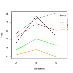
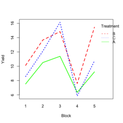
ggplot2 style:
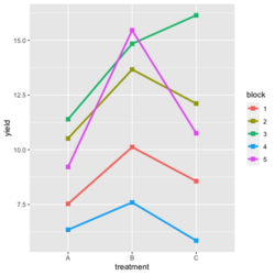


gl(): Generate Factor Levels
Two-way ANOVA
- Interpreting Interactions when Main Effects are Not Significant
- Actually, you can interpret some main effects in the presence of an interaction
- Confusion about Deseq2 wording in the vignette (additive model with main effects only vs interaction)
- Why and When to Include Interactions in a Regression Model
- they have large main effects
- the effect of one changes for various subgroups of the other
- the interaction has been proven in previous studies
- you want to explore new hypotheses
- How to interpret main effects when the interaction effect is not significant?
- When Main Effects are Not Significant, But the Interaction Is. A cross-over interaction.
- Main effects are not significant anymore after adding interaction terms in my linear regression. Frank Harrell answered.
- Can the interaction term of two insignificant coefficients be significant?
- Why does the main effect become not significant when I add an interaction term in a regression model? The interaction effect is more influential in explaining differences in the outcome variable than either the "main effect". moderator
- Including an Interaction term leads to insignificant direct effects. The "main effects" no longer carry the same meaning when an interaction term is included in the model, so their coefficients have no necessary relationship to the coefficients seen by the variables of the same name in a no-interaction model.
- How to Create an Interaction Plot in R? stats::interaction.plot()
An example
devtools::source_gist("https://gist.github.com/arraytools/88449e3c92c752eb7a66ee0189b09606")
dim(df) # [1] 33  3
df[1:2, ]
#          muc6 tumortype    auc
# V1  0.6599192 Carcinoma 0.6056
# V2 12.2342844   sarcoma 0.1858

summary(lm(auc~muc6, data=df))
# Coefficients:
#             Estimate Std. Error t value Pr(>|t|)
# (Intercept)  0.63065    0.05388  11.706 6.56e-13 ***
# muc6        -0.04367    0.01119  -3.903 0.000478 ***
# Residual standard error: 0.2407 on 31 degrees of freedom
# Multiple R-squared:  0.3295,	Adjusted R-squared:  0.3079
# F-statistic: 15.23 on 1 and 31 DF,  p-value: 0.000478

summary(lm(auc~., data=df))
# Coefficients:
#                  Estimate Std. Error t value Pr(>|t|)
# (Intercept)       0.61262    0.07764   7.891 8.32e-09 ***
# muc6             -0.04312    0.01148  -3.758 0.000739 ***
# tumortypesarcoma  0.02846    0.08697   0.327 0.745791
# Residual standard error: 0.2443 on 30 degrees of freedom
# Multiple R-squared:  0.3319,	Adjusted R-squared:  0.2873
# F-statistic: 7.451 on 2 and 30 DF,  p-value: 0.00236

summary(lm(auc~muc6*tumortype, data=df))
# Coefficients:
#                       Estimate Std. Error t value Pr(>|t|)
# (Intercept)            0.53938    0.08281   6.514 3.93e-07 ***
# muc6                  -0.02312    0.01490  -1.552   0.1316
# tumortypesarcoma       0.16194    0.10690   1.515   0.1406
# muc6:tumortypesarcoma -0.04356    0.02198  -1.982   0.0571 .

# Residual standard error: 0.2332 on 29 degrees of freedom
# Multiple R-squared:  0.4116,	Adjusted R-squared:  0.3507
# F-statistic: 6.761 on 3 and 29 DF,  p-value: 0.001352

library(ggplot2); library(magrittr)
df %>% ggplot(aes(muc6, auc, col=tumortype)) +
  geom_point(size=3) +
  geom_smooth(method="lm",se = FALSE)


# Base R plot version
col2 <- c("#F8767D", "#00BFC4") # see my ggplot2 page
col <- col2[as.integer(factor(df$tumortype))]

f$tumortype[1:5]
# [1] "Carcinoma" "sarcoma"   "Carcinoma" "Carcinoma" "sarcoma"
as.integer(factor(df$tumortype))[1:5]
# [1] 1 2 1 1 2

plot(df$muc6, df$auc, col = col, xlab="muc6", ylab="auc", pch=16, cex=1.5)
abline(a = coefs[1], b=coefs[2], col = col2[1], lwd=3)
abline(a = coefs[1] + coefs[3], b = coefs[2] + coefs[4], lty=2, col = col[2], lwd=3)
legend("topright", c("Carcinoma", "sarcoma"), col = col2, lty=1:2, lwd=3)


Type I, II and III Sums of Squares
- Type I, II and III Sums of Squares – the explanation
- type I (sequential): SS(A) for factor A. SS(B | A) for factor B. SS(AB | B, A) for interaction AB. If the data is unbalanced, you will get a different result of using anova(lm(y ~ A * B, data=search)) & anova(lm(y ~ B * A, data=search)). This is default in R.
- type II (ADDED AFTER OTHER MAIN EFFECTS): SS(A | B) for factor A. SS(B | A) for factor B. R's anova().
- type III (ADDED LAST): SS(A | B, AB) for factor A. SS(B | A, AB) for factor B. This is the default in SAS. In R, car:::Anova(, type="III").
- Everything You Always Wanted to Know About ANOVA
- It seems the order does not make a difference in linear regression or Cox regression.
Kruskal-Wallis one-way analysis of variance
- https://en.wikipedia.org/wiki/Kruskal%E2%80%93Wallis_one-way_analysis_of_variance
- The Kruskal-Wallis test and the Wilcoxon test are not the same.
- The Kruskal-Wallis test is used to compare the means of more than two groups, while the Wilcoxon test (also known as the Mann-Whitney U test) is used to compare the means of two groups.
- Both tests are non-parametric and do not assume that the data come from a normal distribution.
- With two samples, a Kruskal-Wallis test is equivalent to a Wilcoxon-Mann-Whitney test but without the direction information; so you lose the ability to do a one-sided test
- How to perform the Kruskal-Wallis test in R?
- Kruskal Wallis test in R-One-way ANOVA Alternative
- Example
mydata <- PlantGrowth
unique(PlantGrowth$group) # [1] ctrl trt1 trt2

# Run Kruskal-Wallis test
kruskal.test(weight ~ group, data = mydata)
#	Kruskal-Wallis rank sum test
#
# data:  weight by group
# Kruskal-Wallis chi-squared = 7.9882, df = 2, p-value = 0.01842
mydata <- PlantGrowth

# Subset data for two groups
groupA <- subset(mydata, group == "ctrl")$weight
groupB <- subset(mydata, group == "trt1")$weight

# Run Wilcoxon-Mann-Whitney test
wilcox.test(groupA, groupB)

#	Wilcoxon rank sum test with continuity correction
#
# data:  groupA and groupB
# W = 67.5, p-value = 0.1986
# alternative hypothesis: true location shift is not equal to 0
#
# Warning message:
# In wilcox.test.default(groupA, groupB) :
#   cannot compute exact p-value with ties
Multilevel, Simpson paradox
Multilevel Correlations: A New Method for Common Problems. Simpson paradox.
ANCOVA
MANOVA
- MANOVA(Multivariate Analysis of Variance) using R
- MANOVA in R – How To Implement and Interpret One-Way MANOVA