File:Filtered p.png
Jump to navigation
Jump to search

Size of this preview: 558 × 600 pixels. Other resolution: 1,020 × 1,096 pixels.
Original file (1,020 × 1,096 pixels, file size: 171 KB, MIME type: image/png)
Summary
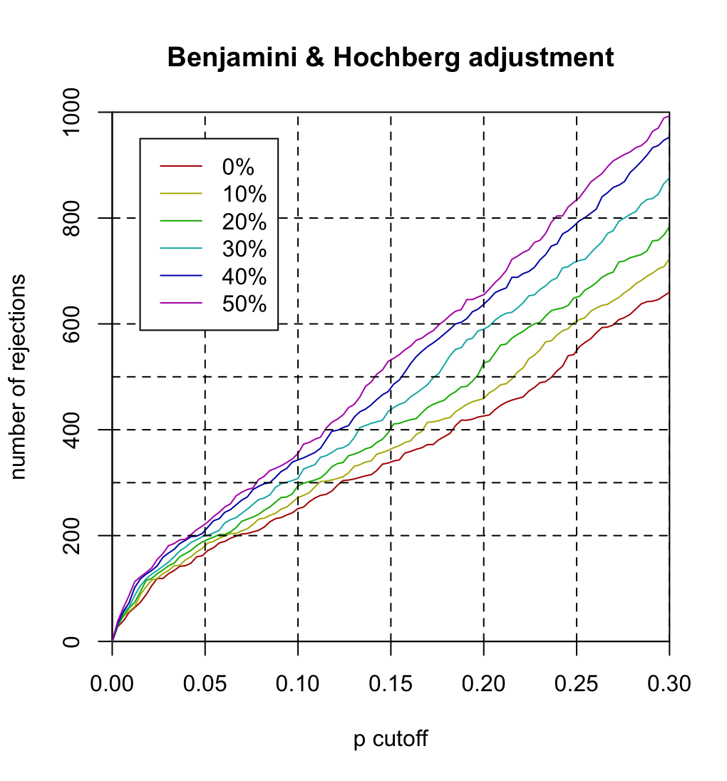
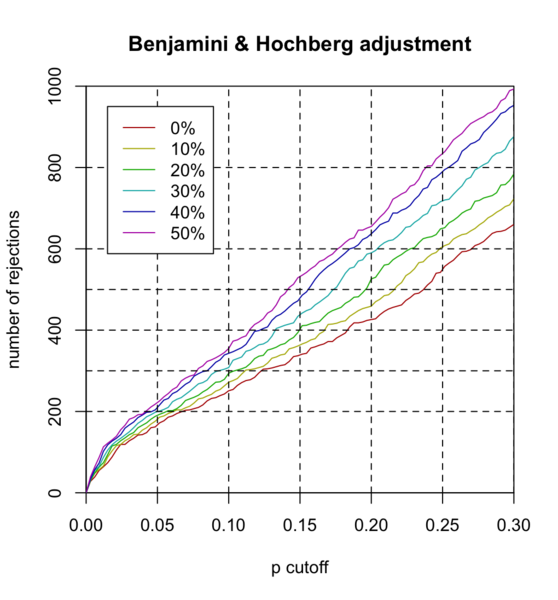
Note:
- x-axis "p cutoff" should be "BH cutoff" or "FDR cutoff".
- Each curve represents theta (filtering threshold). For example, theta=.1 means 10% of genes are filtered out before we do multiple testing (or BH adjustment).
- It is seen the larger the theta, the more hypotheses are rejected at the same FDR cutoff. For example,
- if theta=0, 251 hypotheses are rejected at FDR=.1
- if theta=.5, 355 hypotheses are rejected at FDR=.1.
BiocManager::install("ALL")
library("ALL")
library(genefilter)

data("ALL")
bcell <- grep("^B", as.character(ALL$BT))
moltyp <- which(as.character(ALL$mol.biol) %in%
                    +                     c("NEG", "BCR/ABL"))
ALL_bcrneg <- ALL[, intersect(bcell, moltyp)]
ALL_bcrneg$mol.biol <- factor(ALL_bcrneg$mol.biol)
table(ALL_bcrneg$mol.biol)

S2 <- rowVars(exprs(ALL_bcrneg))
p2 <- rowttests(ALL_bcrneg, "mol.biol")$p.value
theta <- seq(0, .5, .1)
# The filtered_p function permits easy simultaneous calculation of unadjusted
#   or adjusted p-values over a range of filtering thresholds (θ).
p_bh <- filtered_p(S2, p2, theta, method="BH")
dim(p_bh)
# [1] 12625     6
head(p_bh) # adjusted p-values using the BH method
#             0%       10%       20%       30%       40%       50%
# [1,] 0.9185626 0.8943104 0.8624798 0.8278077        NA        NA
# [2,] 0.9585758 0.9460504 0.9304104 0.9059466 0.8874485 0.8709793
# [3,] 0.7022442        NA        NA        NA        NA        NA
# [4,] 0.9806216 0.9747555 0.9680574 0.9567131        NA        NA
# [5,] 0.9506087 0.9349386 0.9123998 0.8836386        NA        NA
# [6,] 0.6339004 0.5896890 0.5440851 0.4951371 0.4497915 0.4102711

range(p.adjust(p2, "BH") - p_bh[,1]) # 0 0

apply(p_bh, 2, function(x) mean(is.na(x))) |> round(2)
#   0% 10% 20% 30% 40% 50%
#  0.0 0.1 0.2 0.3 0.4 0.5

i <- order(S2, decreasing = T)
i2 <- sort(i[1:round(12625*.9)])
# [1] 1 2 4 5 6  # sort the 3rd gene is filtered out
tmp <- rep(NA, 12625); tmp[i2] <- p.adjust(p2[i2], "BH")
range(tmp - p_bh[, 2], na.rm = TRUE) # 0 0

i3 <- sort(i[1:round(12625*.8)]); i3[1:5]
# [1] 1 2 4 5 6
tmp <- rep(NA, 12625); tmp[i3] <- p.adjust(p2[i3], "BH")
range(tmp - p_bh[, 3], na.rm = TRUE) # 0 0

i4 <- sort(i[1:round(12625*.7)]); i4[1:5]
# [1] 1 2 4 5 6
tmp <- rep(NA, 12625); tmp[i4] <- p.adjust(p2[i4], "BH")
range(tmp - p_bh[, 4], na.rm = TRUE) # [1] -6.533250e-05  9.570921e-05

i5 <- sort(i[1:round(12625*.6)]); i5[1:5]
# [1]  2  6  8  9 10
tmp <- rep(NA, 12625); tmp[i5] <- p.adjust(p2[i5], "BH")
range(tmp - p_bh[, 5], na.rm = TRUE) # 0 0

i6 <- sort(i[1:round(12625*.5)]); i6[1:5]
# [1]  2  6  8  9 10
tmp <- rep(NA, 12625); tmp[i6] <- p.adjust(p2[i6], "BH")
range(tmp - p_bh[, 6], na.rm = TRUE) # [1] -0.0000171919  0.0002731363

# input p_bh is already FDR adjusted p-values
rejection_plot(p_bh, at="sample",
               xlim=c(0,.3), ylim=c(0,1000),
               main="Benjamini & Hochberg adjustment")
sapply(c(.05, .1, .15, .2, .25, .3), function(x) sum(p_bh[,1] < x))
# 169 251 341 426 554 660
sapply(c(.05, .1, .15, .2, .25, .3), function(x) sum(p_bh[,2] < x, na.rm=T))
# 178 272 363 459 602 723
sapply(c(.05, .1, .15, .2, .25, .3), function(x) sum(p_bh[,3] < x, na.rm=T))
# 192 294 402 526 649 784
sapply(c(.05, .1, .15, .2, .25, .3), function(x) sum(p_bh[,4] < x, na.rm=T))
# 201 308 439 590 717 876
sapply(c(.05, .1, .15, .2, .25, .3), function(x) sum(p_bh[,5] < x, na.rm=T))
# 209 343 475 637 788 953
sapply(c(.05, .1, .15, .2, .25, .3), function(x) sum(p_bh[,6] < x, na.rm=T))
# 222 355 530 655 836 993

abline(h=200, lty=2); abline(v=.05, lty=2)
abline(h=300, lty=2); abline(v=.1, lty=2)
abline(h=400, lty=2); abline(v=.15, lty=2)
abline(h=500, lty=2); abline(v=.2, lty=2)
abline(h=600, lty=2); abline(v=.25, lty=2)
abline(h=800, lty=2); abline(v=.3, lty=2)
File history
Click on a date/time to view the file as it appeared at that time.
| Date/Time | Thumbnail | Dimensions | User | Comment | |
|---|---|---|---|---|---|
| current | 21:35, 11 March 2024 | | 1,020 × 1,096 (171 KB) | Brb (talk | contribs) | Note: # x-axis "p cutoff" should be "BH cutoff" or "FDR cutoff". # Each curve represents theta (filtering threshold). For example, theta=.1 means 10% of genes are filtered out before we do multiple testing (or BH adjustment). # It is seen the larger the theta, the more hypotheses are rejected at the same FDR cutoff. For example, #* if theta=0, 251 hypotheses are rejected at FDR=.1 #* if theta=.5, 355 hypotheses are rejected at FDR=.1. <syntaxhighlight lang='r'> BiocManager::install("ALL")... |
You cannot overwrite this file.
File usage
The following page uses this file: