File:Wgcna 3clusters dend.png

Summary

# WGCNA uses standard hierarchical clustering (specifically the hclust function in R), 
# but the "magic" that makes it WGCNA is the Topological Overlap Matrix (TOM) used as the distance metric.

# https://en.wikipedia.org/wiki/Weighted_correlation_network_analysis
# https://cloud.wikis.utexas.edu/wiki/spaces/bioiteam/pages/47714689/Clustering+using+WGCNA
# https://ngs101.com/how-to-build-gene-co-expression-networks-from-rna-seq-data-using-wgcna-complete-step-by-step-guide-for-absolute-beginners/
# https://edo98811.github.io/WGCNA_official_documentation/
# https://www.reddit.com/r/bioinformatics/comments/1cr7m9j/what_happened_to_the_wgcna_tutorial/

# -------------------------
library(WGCNA)

# Set seed for reproducibility
set.seed(123)

# 1. Create a "Scaffold" for 3 modules (patterns of expression)
nSamples = 50
pattern1 = rnorm(nSamples)
pattern2 = rnorm(nSamples)
pattern3 = rnorm(nSamples)

# 2. Generate 1000 genes based on these patterns + some noise
# Module 1: 200 genes correlated with pattern 1
mod1 = matrix(rep(pattern1, 200), nrow=nSamples) + matrix(rnorm(nSamples*200, sd=0.5), nrow=nSamples)
# Module 2: 200 genes correlated with pattern 2
mod2 = matrix(rep(pattern2, 200), nrow=nSamples) + matrix(rnorm(nSamples*200, sd=0.5), nrow=nSamples)
# Module 3: 200 genes correlated with pattern 3
mod3 = matrix(rep(pattern3, 200), nrow=nSamples) + matrix(rnorm(nSamples*200, sd=0.5), nrow=nSamples)
# Noise: 400 random genes
noise = matrix(rnorm(nSamples*400), nrow=nSamples)

# 3. Combine into one expression matrix (Samples as Rows, Genes as Columns)
datExpr = as.data.frame(cbind(mod1, mod2, mod3, noise))
colnames(datExpr) = paste0("Gene", 1:1000)
rownames(datExpr) = paste0("Sample", 1:50)

# Check dimensions (Should be 50 x 1000)
print(dim(datExpr))

# Choose Soft Threshold
powers = c(c(1:10), seq(from = 12, to=30, by=2))
sft = pickSoftThreshold(datExpr, powerVector = powers, verbose = 3)

# Plotting the results (Scale-Free Topology)
# you should see the $R^2$ curve rise quickly.
# The curve should hit a plateau (usually above 0.8 or 0.9) at a relatively low power (like 6 or 8).
# See "WGCNA: an R package for weighted gene co-expression network analysis,"
# Official WGCNA FAQ and Documentation https://edo98811.github.io/WGCNA_official_documentation/faq.html
#   says for more than 40 samples, power=6 for Unsigned and signed hybrid networks	
#                                  power=12 for Signed networks
# Choose signed network, if I want to see separate modules for upregulated genes and downregulated genes.
# For signed network, modules are easier to interpret because all genes in a cluster move together.
# Strongly recommended in later documentation for better biological accuracy.
# Verdict: 
#   If you are studying a disease vs. control and want to know which genes are 
#   "activated" as a functional unit, choose Signed. If you just want to find 
#   any genes that are mathematically related regardless of direction, stay with Unsigned.

# Check the power suggested by the package
sft$powerEstimate # NA
# If sft$powerEstimate returns NA, it means the data never hit the internal default threshold (usually 0.90)

plot(sft$fitIndices[,1], -sign(sft$fitIndices[,3])*sft$fitIndices[,2],
     xlab="Soft Threshold (power)", ylab="Scale Free Topology Model Fit,signed R^2",
     type="n", main = "Scale Independence")
text(sft$fitIndices[,1], -sign(sft$fitIndices[,3])*sft$fitIndices[,2],
     labels=powers, col="red")

# Even at power 10, your model fit is only at 0.25. 
# In a successful WGCNA run, you want that value on the y-axis to be near 0.80.

# the "Scale-Free Topology" fit is finally behaving. It reached the magic threshold of 0.80 at power 30.

# Typically, for 50 samples, WGCNA authors suggest a power around 6 (for unsigned networks) or 12 (for signed networks).
# The fact that you need 30 suggests that the "Noise" we added in the simulation is very strong relative to the "Signals."
pow <- 12
net = blockwiseModules(datExpr, power = pow, TOMType = "signed", 
                       minModuleSize = 30, reassignThreshold = 0, 
                       mergeCutHeight = 0.25, numericLabels = TRUE, 
                       pamRespectsDendro = FALSE, verbose = 3)
# names(net)
# [1] "colors"         "unmergedColors" "MEs"            "goodSamples"   
# [5] "goodGenes"      "dendrograms"    "TOMFiles"       "blockGenes"    
# [9] "blocks"         "MEsOK"      

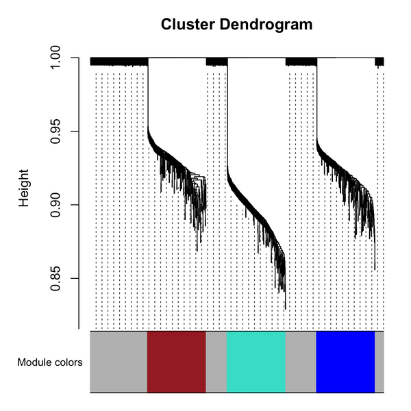
# Visualize the clusters
moduleColors = labels2colors(net$colors)
plotDendroAndColors(net$dendrograms[[1]], moduleColors[net$blockGenes[[1]]],
                    "Module colors", dendroLabels = FALSE, hang = 0.03,
                    addGuide = TRUE, guideHang = 0.05)

# 0 is always the unassigned/grey module.
table(net$colors)
#   0   1   2   3 
# 400 200 200 200 

# Module Label	Color	Number of Genes	Interpretation
#      1	      Turquoise	~200	Your first simulated functional group.
#      2	      Blue	~200	Your second simulated functional group.
#      3	      Brown	~200	Your third simulated functional group.
#      0	      Grey	~400	The Noise. Genes that didn't correlate.

# Module Eigengene (ME) is defined as the first principal component of the expression matrix for a given module, rather than a simple arithmetic average.
dim(net$MEs) # Module Eigengene
# [1] 50  4
# 1. Identify which ME corresponds to the Turquoise module
# (Usually ME1 or MEturquoise)
me_to_plot = net$MEs$ME1  # If using numeric labels, or MEturquoise if colors

# 2. Plot the Eigengene (The "Summary") against the Pattern (The "Truth")
op <- par(mfrow = c(2,1), mar = c(4,4,2,1))

# Plot the original pattern we simulated
plot(pattern1, type="l", col="red", lwd=2, main="Original Simulated Pattern", ylab="Expression")

# Plot the Module Eigengene found by WGCNA
plot(me_to_plot, type="l", col="turquoise", lwd=2, main="WGCNA Module Eigengene", ylab="ME Value")
par(op)

# Heatmap of turquoise genes and all samples
# A good module will show a clear, consistent block of color where all genes are moving in sync.
# You should see vertical "stripes" of red (high expression) and blue (low expression). Because these genes were all simulated from the same pattern, they should all "flash" red or blue at the same time across the samples.
# 1. Select the genes
which_module = "turquoise" 
module_genes = colnames(datExpr)[moduleColors == which_module]

# 2. Prepare the matrix (Genes as rows, Samples as columns)
# We scale the data so genes with high vs low expression are comparable
plot_matrix = t(scale(datExpr[, module_genes])) # genes x samples

# 3. Plot using base heatmap
# A standard Red-White-Blue palette
my_palette = colorRampPalette(c("blue", "white", "red"))(n = 100)

heatmap(plot_matrix, 
        Rowv = NA, 
        Colv = NA, 
        col = my_palette, 
        scale = "none", # We already scaled manually
        main = paste("Expression Pattern of", which_module))

# Visualize the correlation matrix.
# Calculate correlation between all Module Eigengenes
inst_cor = cor(net$MEs)

# Plot the relationship between modules
heatmap(inst_cor, 
        col = my_palette, 
        symm = TRUE,      # The matrix is symmetrical
        main = "Inter-Module Correlation")

# identify genes have the highest correlation to the Module Eigengene.
# In WGCNA, this correlation is known as Module Membership (kME). 
# It is also frequently called Intramodular Connectivity.
# A gene with a high kME (close to 1.0) is considered a Hub Gene. 
# These are the "influencers" of the module—if the Hub Gene is expressed,
# the rest of the module is almost certainly expressed too
# 1. Calculate the kME (Module Membership)
# You can calculate the correlation between every gene in your dataset and every Module Eigengene (ME).
 # 1. Calculate correlations (kME)
 # 'datExpr' has genes as columns, 'net$MEs' has Eigengenes as columns
 geneModuleMembership = as.data.frame(cor(datExpr, net$MEs, use = "p"))
 # 2. Add P-values to see if the correlation is statistically significant
 MMPvalue = as.data.frame(corPvalueStudent(as.matrix(geneModuleMembership), nSamples = nrow(datExpr)))
 # Rename columns for clarity
 names(geneModuleMembership) = paste0("kME", names(net$MEs))
 names(MMPvalue) = paste0("p.kME", names(net$MEs))

# 2. Identify the Top Hub Genes for a Specific Module
# Let's say you want to find the "leaders" of the Turquoise module (usually ME1).
 # Define the module you are interested in
 column = "kMEME1" # Adjust based on your net$MEs names (e.g., kMEturquoise)
 
 # 1. Subset the data to only look at genes assigned to that module
 module_genes_info = geneModuleMembership[net$colors == 1, ] # Using numeric 1 for Turquoise
 
 # 2. Sort the genes by their kME value in descending order
 hub_genes = module_genes_info[order(-module_genes_info[[column]]), , drop = FALSE]
 
 # 3. View the top 10 Hub Genes
 head(hub_genes, 10)
 
# 3. Visualizing kME: The "Hub" Plot
# A common way to visualize this is to plot the Gene Significance 
# (correlation with a trait) vs. Module Membership. 
# Since we are using simulated data without a trait, 
# we can simply plot the kME values to see the distribution.
 # Histogram of kME values for the Turquoise module
 hist(hub_genes[[column]], 
      breaks = 20, 
      col = "turquoise", 
      main = "Distribution of kME in Turquoise Module",
      xlab = "Module Membership (Correlation to Eigengene)")