Uploads by Brb
This special page shows all uploaded files.
| Date | Name | Thumbnail | Size | Description | Versions |
|---|---|---|---|---|---|
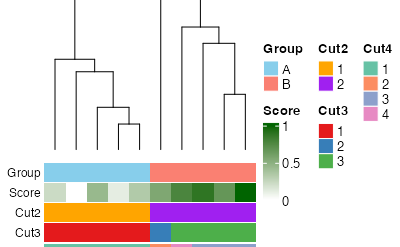
| 10:48, 1 December 2025 | Dendro colorbars.png (file) |  |
11 KB | <syntaxhighlight lang='r'> library(ComplexHeatmap) library(circlize) library(RColorBrewer) set.seed(123) # --- Example data (10 samples) --- mat <- matrix(rnorm(30), nrow = 10) rownames(mat) <- paste0("Sample", 1:10) mat[1:5, ] <- mat[1:5, ] mat[6:10, ] <- mat[6:10, ] + 2 # Cluster on samples (rows) hc <- hclust(dist(mat)) # Annotations in ORIGINAL sample order groups <- rep(c("A", "B"), each = 5) score <- seq(0, 1, length = 10) cl2 <- cutree(hc, 2) cl3 <- cutree(hc, 3) cl4 <- cutree(hc,... | 1 |
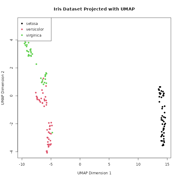
| 17:16, 10 November 2025 | Umap-iris.png (file) |  |
25 KB | <syntaxhighlight lang='r'> library(umap) # Load the built-in Iris dataset data(iris) # Separate the features (variables) from the species labels iris_features <- iris[, 1:4] iris_species <- iris[, 5] # Run UMAP, reducing the 4 dimensions down to 2 # n_neighbors: Controls how UMAP balances local vs. global structure. # min_dist: Controls how tightly points are packed together. iris_umap_results <- umap(iris_features, random_state = 42) # The result is a list. The actual 2D coordinates are... | 1 |
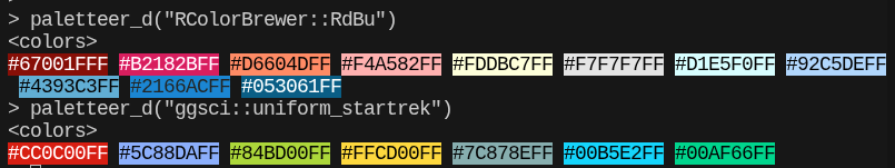
| 19:07, 28 October 2025 | Paletteer d.png (file) | 39 KB | <syntaxhighlight lang='r'> paletteer_d("RColorBrewer::RdBu") #<colors> #67001FFF #B2182BFF #D6604DFF #F4A582FF #FDDBC7FF #F7F7F7FF #D1E5F0FF #92C5DEFF #4393C3FF #2166ACFF #053061FF paletteer_d("ggsci::uniform_startrek") # <colors> #CC0C00FF #5C88DAFF #84BD00FF #FFCD00FF #7C878EFF #00B5E2FF #00AF66FF </syntaxhighlight> | 1 | |
| 15:12, 4 October 2025 | Massage.png (file) |  |
1.55 MB | 1 | |
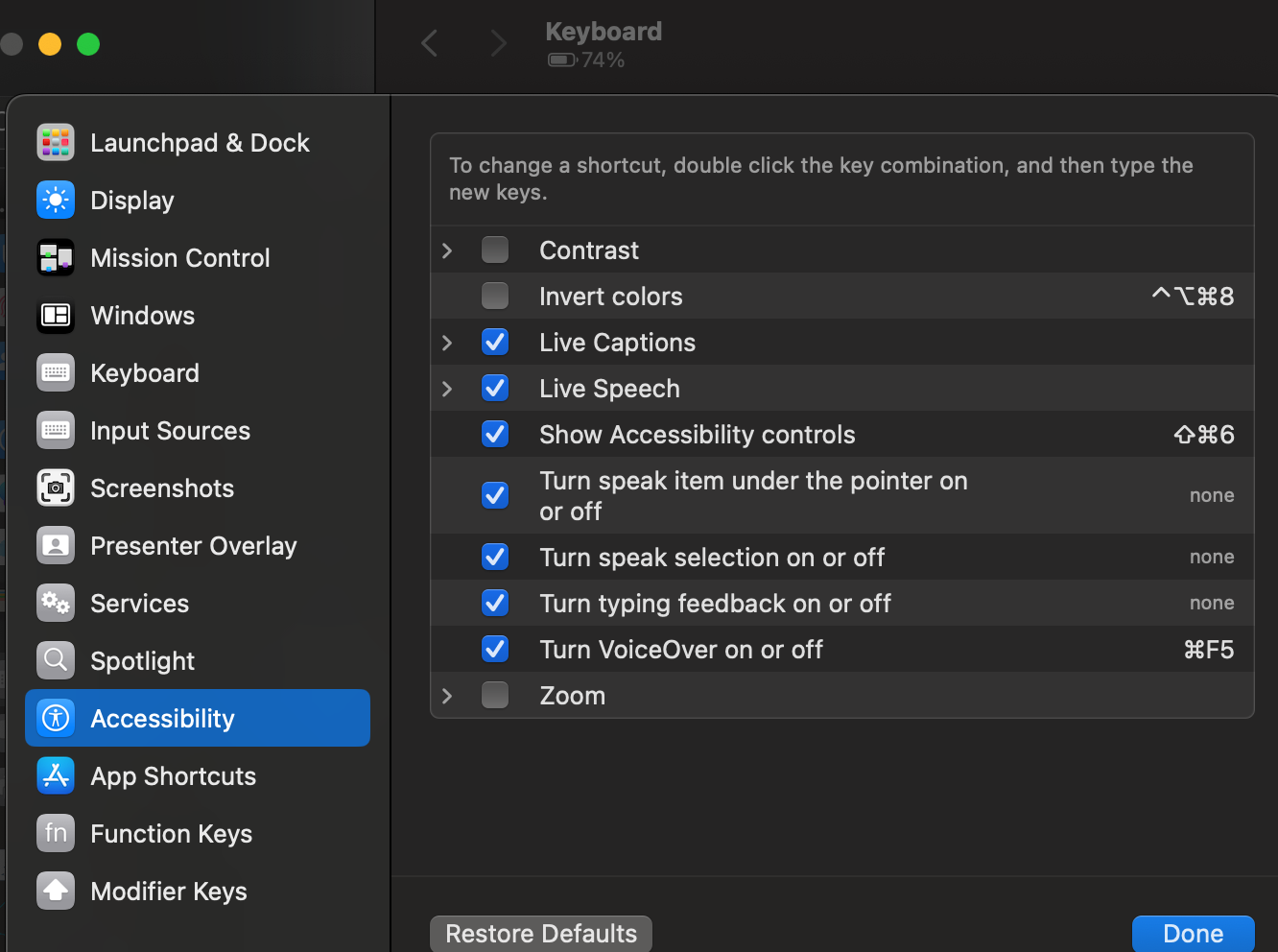
| 14:57, 8 September 2025 | MacSettingKeyboardShortcut.png (file) |  |
274 KB | 1 | |
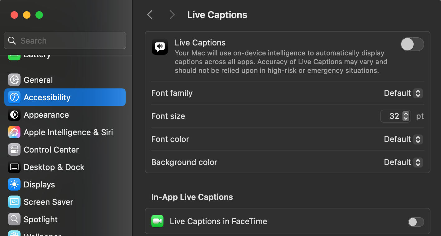
| 14:56, 8 September 2025 | MacSettingLiveCaption.png (file) |  |
271 KB | 1 | |
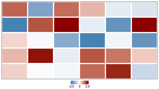
| 09:17, 7 August 2025 | Heatmap-gaps.png (file) |  |
4 KB | <syntaxhighlight lang='r'> # 1. Prepare the data set.seed(42) mat = matrix(rnorm(30, mean = 0, sd = 1.2), nrow = 5, ncol = 6) mat[2, 1] = -2.5 mat[2, 6] = 2.5 mat[1, 2] = -1.8 mat[4, 4] = 1.8 # 2. Define the color palette library(circlize) col_fun = colorRamp2(c(-2.5, 0, 2.5), c("steelblue", "white", "darkred")) # 3. Create the heatmap object library(ComplexHeatmap) ht = Heatmap( mat, col = col_fun, cluster_rows = FALSE, cluster_columns = FALSE, show_row_names = FALSE, show_colu... | 1 |
| 14:18, 29 July 2025 | Inkscape-heatmap.svg (file) |  |
7 KB | 1 | |
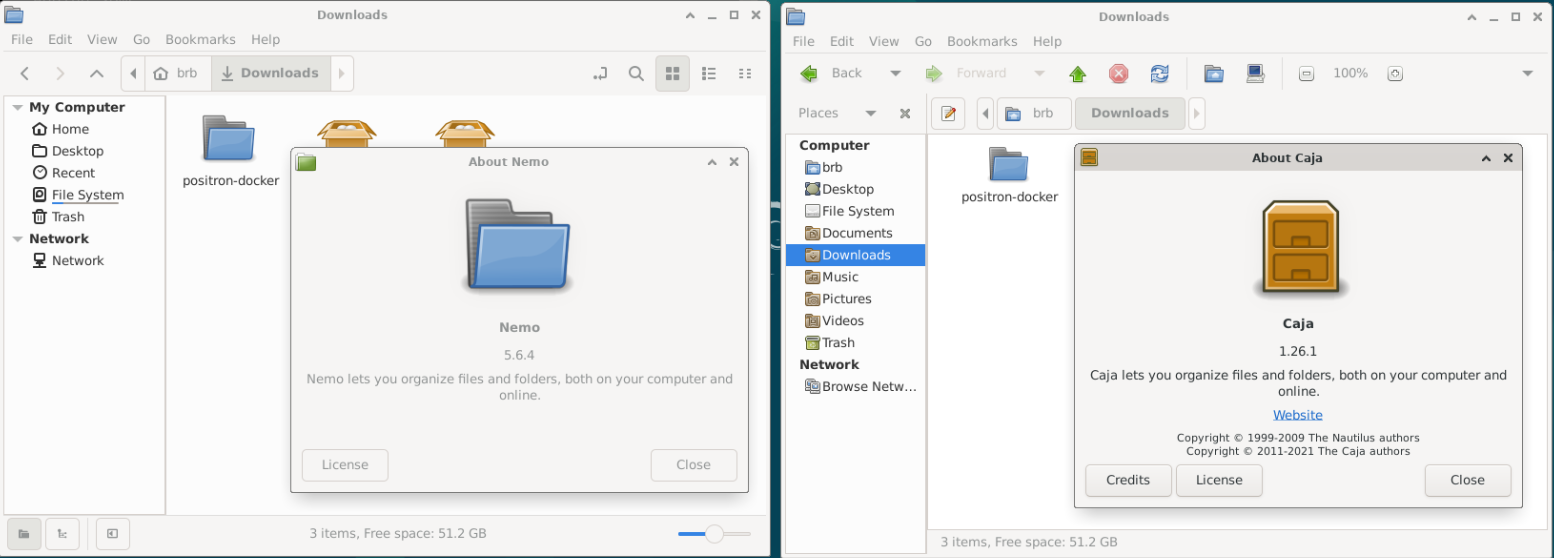
| 08:16, 19 July 2025 | NemoCaja.png (file) |  |
182 KB | 1 | |
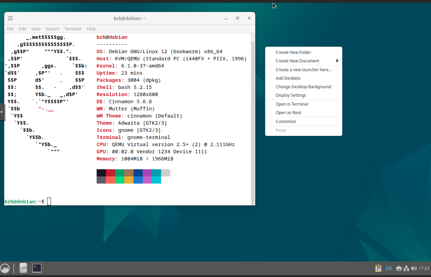
| 16:25, 5 July 2025 | Cinnamon.png (file) |  |
290 KB | 1 | |
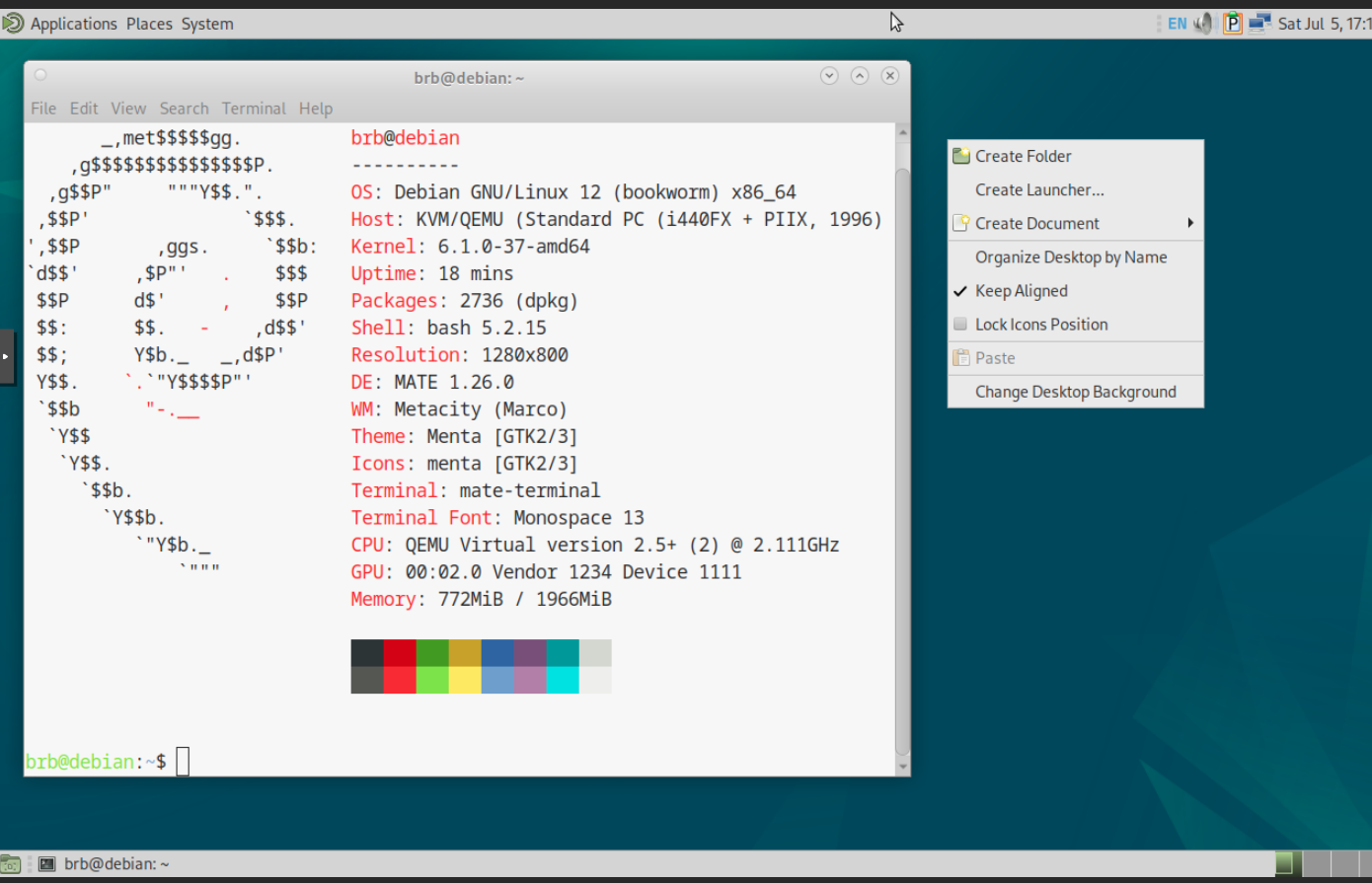
| 16:18, 5 July 2025 | MATE.png (file) |  |
296 KB | 1 | |
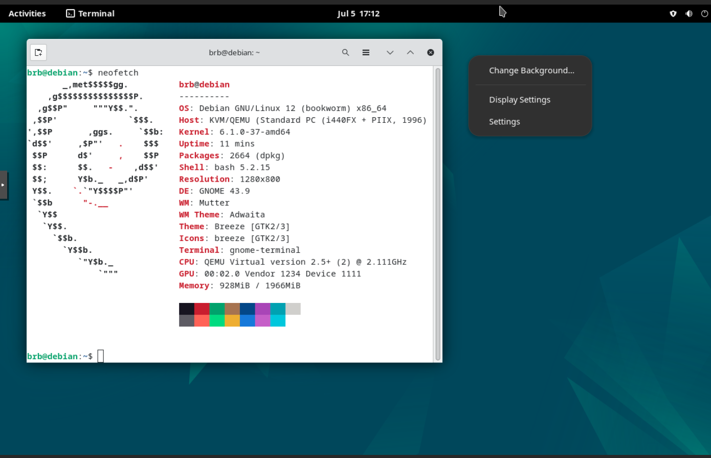
| 16:13, 5 July 2025 | GNOME.png (file) |  |
273 KB | 1 | |
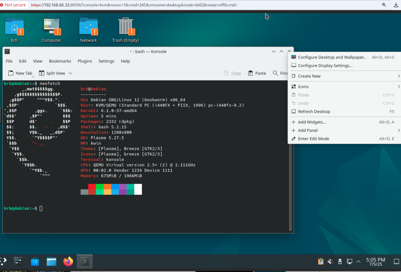
| 16:06, 5 July 2025 | KDE.png (file) |  |
325 KB | 1 | |
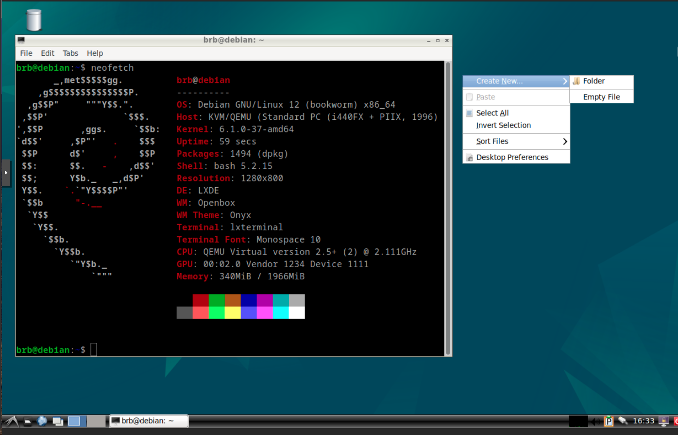
| 15:52, 5 July 2025 | LXDE.png (file) |  |
251 KB | 1 | |
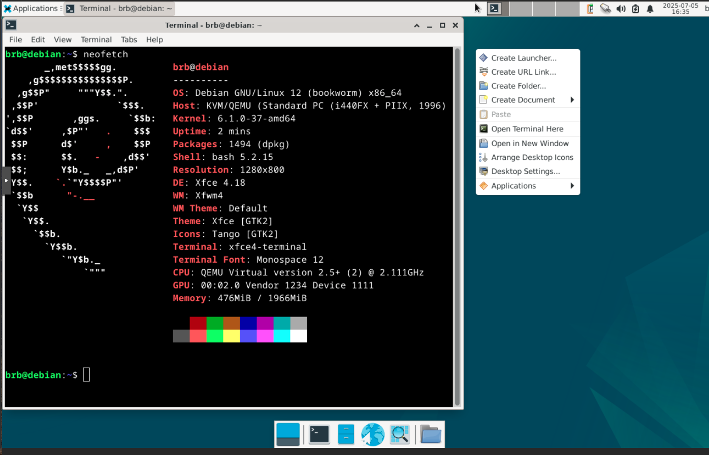
| 15:52, 5 July 2025 | Xfce.png (file) |  |
274 KB | 1 | |
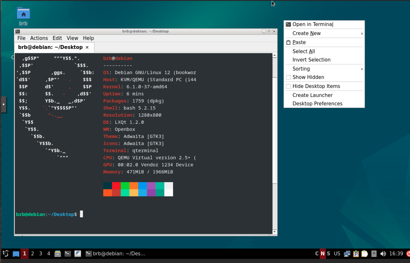
| 15:50, 5 July 2025 | LXQt.png (file) |  |
271 KB | 1 | |
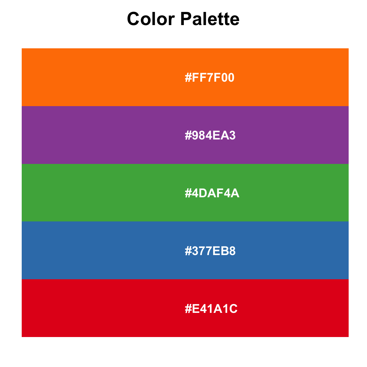
| 14:16, 2 July 2025 | Palbarplot.png (file) |  |
57 KB | 1 | |
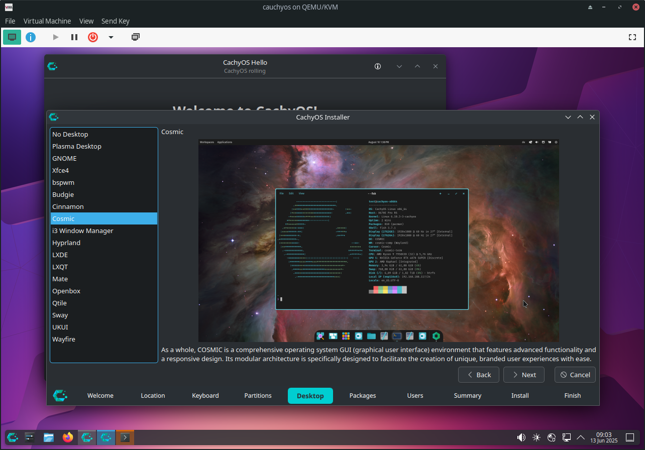
| 08:07, 13 June 2025 | Cauchyos install.png (file) |  |
579 KB | 1 | |
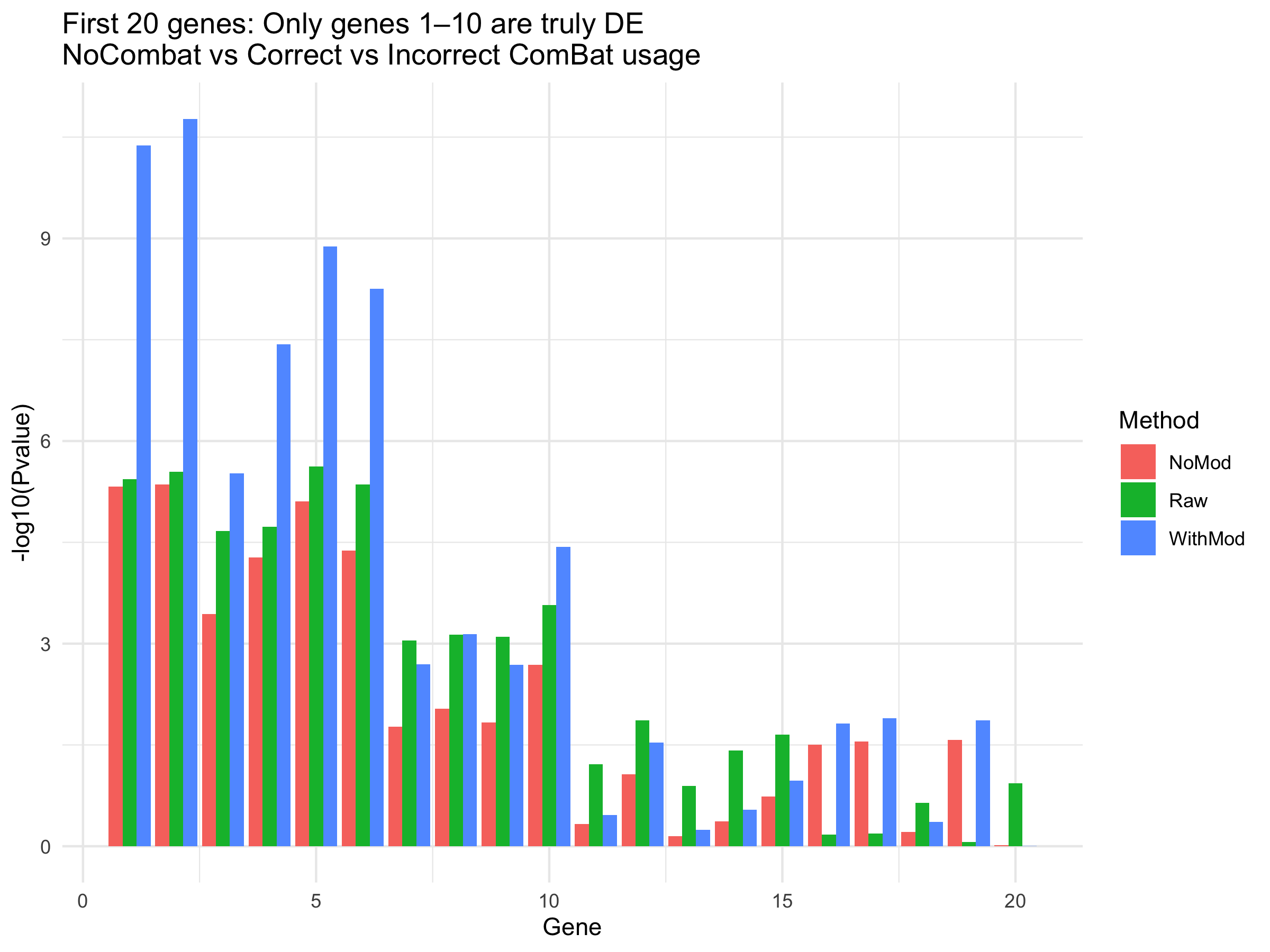
| 12:44, 20 May 2025 | Combat DE mod.png (file) |  |
149 KB | Demonstrate the importance of the 'mod' parameter in sva::ComBat() <syntaxhighlight lang='r'> library(sva) library(limma) library(ggplot2) library(tidyr) set.seed(42) n_genes <- 100 n_samples <- 20 # Group: 10 Case and 10 Control — spread across batches group <- sample(rep(c("Control", "Case"), each=10)) # now randomized batch <- rep(c(1, 2), each=10) # Simulate expression data expr <- matrix(rnorm(n_genes * n_samples, mean=5, sd=1), nrow=n_genes) # Add true signal to 10 genes for Case... | 1 |
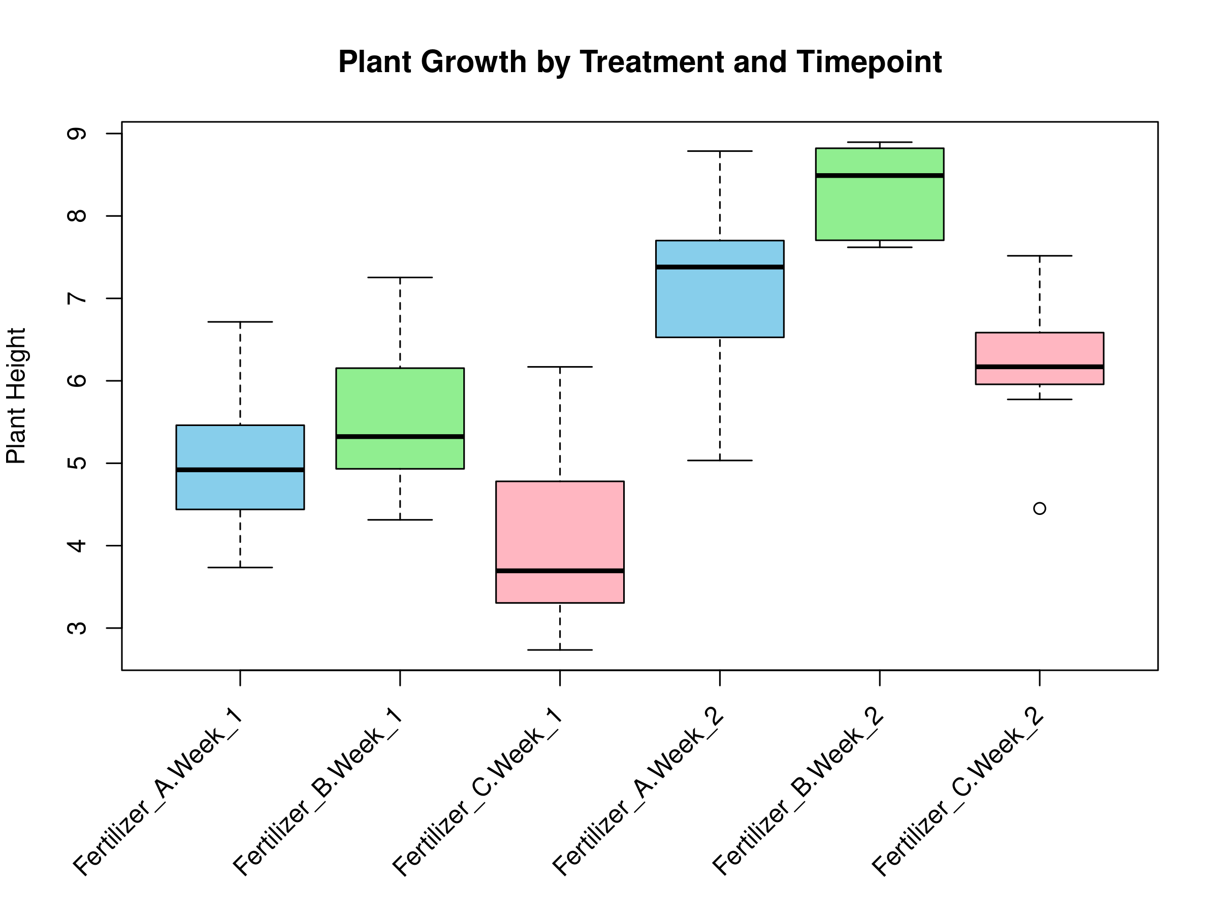
| 20:47, 17 May 2025 | Twoway.png (file) |  |
76 KB | <syntaxhighlight lang='r'> png("~/Downloads/twoway.png", width=8, height=6, units="in",res=300) par(mar = c(8, 4, 4, 2)) boxplot(y ~ treatment * timepoint, data = df, col = c("skyblue", "lightgreen", "lightpink"), main = "Plant Growth by Treatment and Timepoint", xlab = "", ylab = "Plant Height", xaxt = "n") # Add rotated x-axis labels labels <- levels(interaction(df$treatment, df$timepoint)) axis(1, at = 1:length(labels), labels = FALSE) # Add ticks without labels... | 1 |
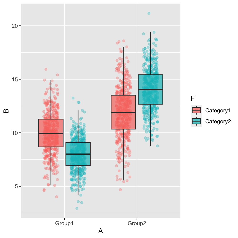
| 12:33, 17 April 2025 | Groupjitterboxplot.png (file) |  |
247 KB | <syntaxhighlight lang='r'> library(ggplot2) library(dplyr) # Create a sample dataset with large sample size set.seed(42) n_per_group <- 500 # 500 samples per group and category combination (2000 total) data <- data.frame( A = rep(c("Group1", "Group2"), each = n_per_group * 2), B = c(rnorm(n_per_group, 10, 2), rnorm(n_per_group, 8, 1.5), # Group1: Category1, Category2 rnorm(n_per_group, 12, 2.5), rnorm(n_per_group, 14, 2)), # Group2: Category1, Category2 F = rep(rep(c("Categ... | 1 |
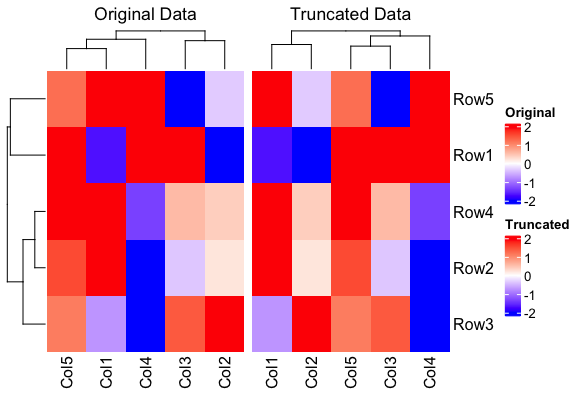
| 16:37, 31 January 2025 | Heatmapcolparam.png (file) |  |
27 KB | <syntaxhighlight lang='r'> library(ComplexHeatmap) library(circlize) # Create a sample 5x5 matrix with values from -4 to 4 set.seed(123) # for reproducibility example_matrix <- matrix(runif(25, -4, 4), nrow = 5) colnames(example_matrix) <- paste0("Col", 1:5) rownames(example_matrix) <- paste0("Row", 1:5) # Define the color function that truncates at -2 and 2 col_fun <- colorRamp2(c(-2, 0, 2), c("blue", "white", "red")) # Plot the heatmap without truncating the data heatmap1 <- Heatmap(exa... | 1 |
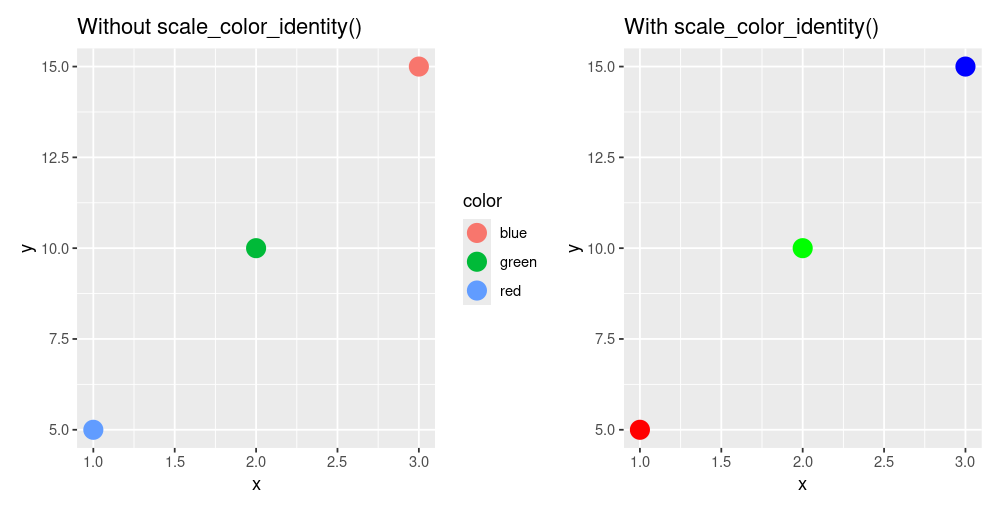
| 18:37, 11 January 2025 | Scale color identity.png (file) |  |
24 KB | 2 | |
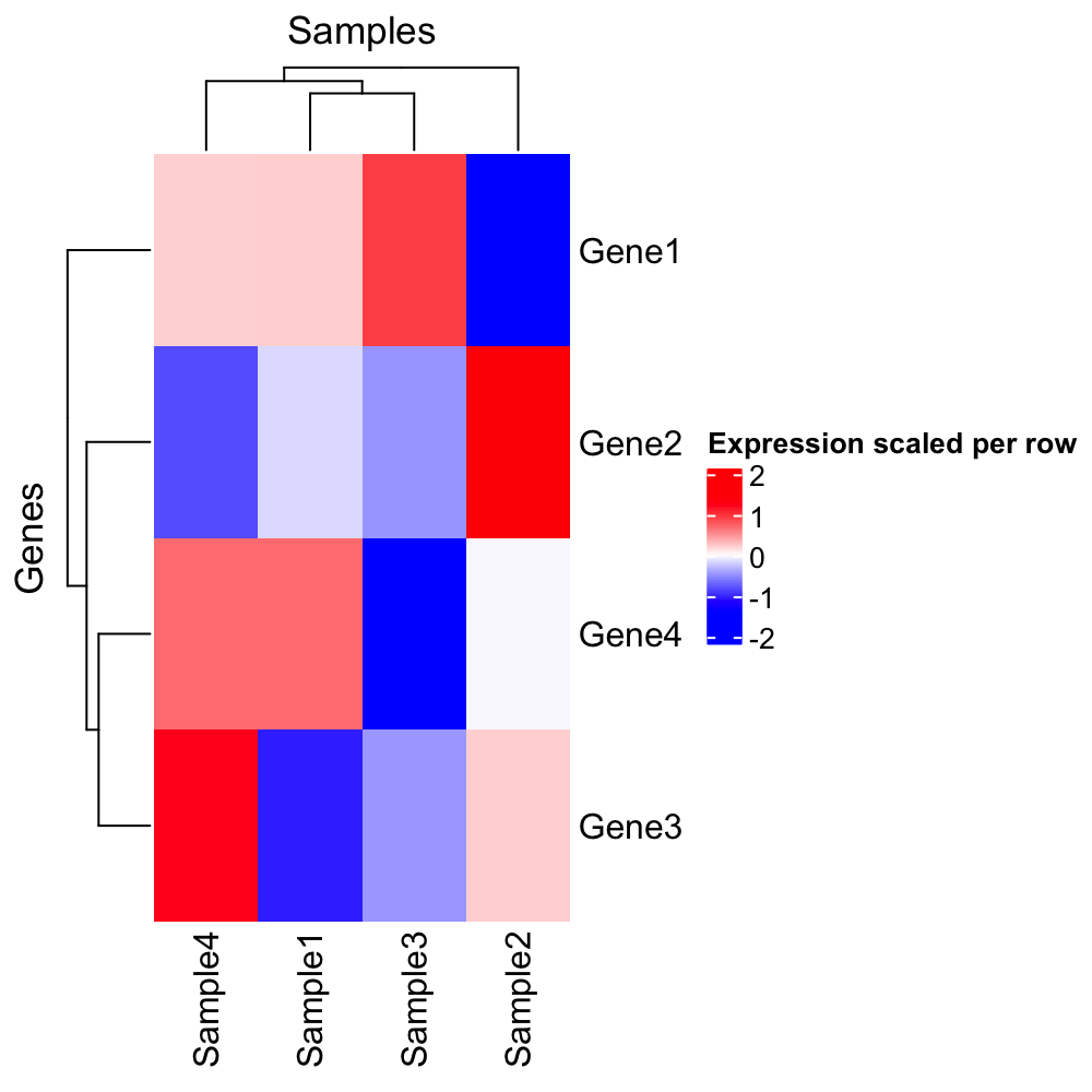
| 20:27, 26 December 2024 | Hmscaled.png (file) |  |
61 KB | 2 | |
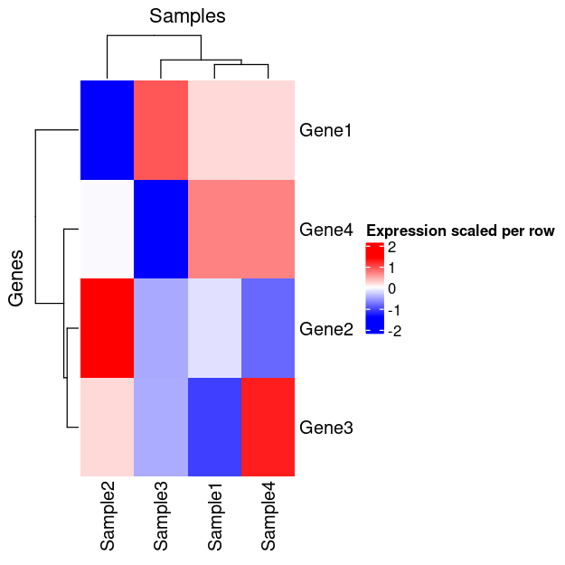
| 20:21, 26 December 2024 | Hmscaled2.png (file) |  |
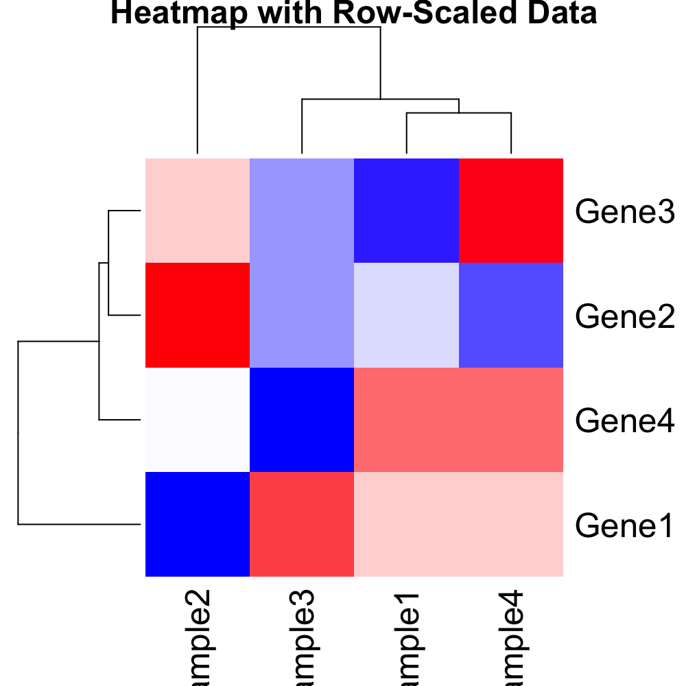
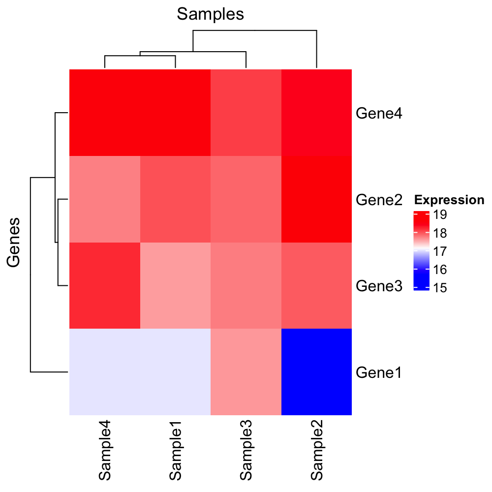
21 KB | <syntaxhighlight lang='r'> x <- structure(c(16.9966943817533, 17.9931011170293, 17.5792623673341, 18.5768638712856, 15.6183559348761, 18.605802884533, 17.9288112453195, 18.4134150861349, 17.6070787425032, 17.8698729193728, 17.7444512372316, 18.092093724098, 16.9949257540877, 17.7299728705232, 18.2145767113386, 18.5766893731416), dim = c(4L, 4L), dimnames = list(c("Gene1", "Gene2", "Gene3", "Gene4"), c("Sample1", "Sample2", "Sample3","Sample4"))) scaled_x <- t(sca... | 1 |
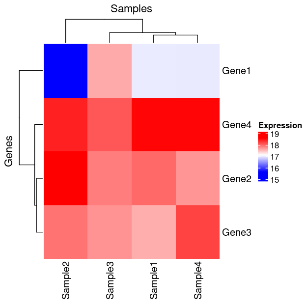
| 20:20, 26 December 2024 | Hmx2.png (file) |  |
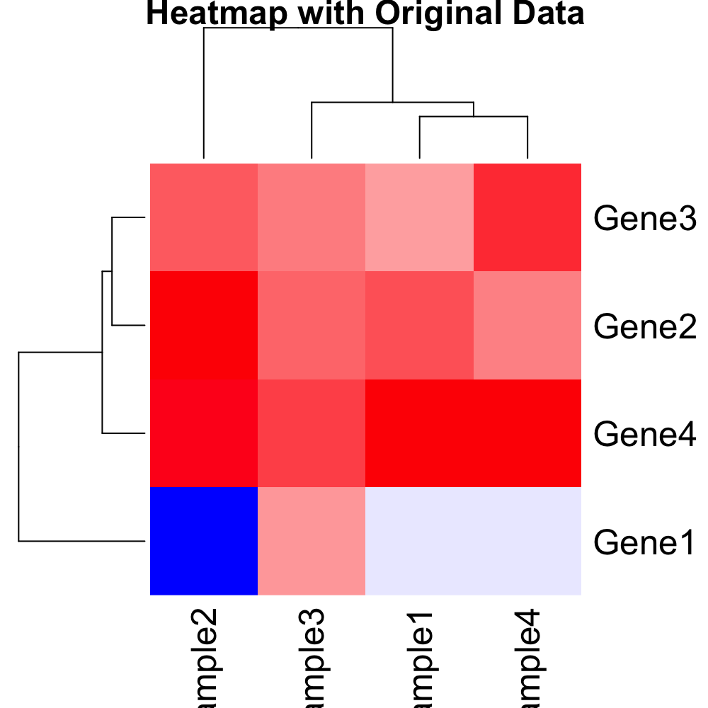
20 KB | <syntaxhighlight lang='r'> x <- structure(c(16.9966943817533, 17.9931011170293, 17.5792623673341, 18.5768638712856, 15.6183559348761, 18.605802884533, 17.9288112453195, 18.4134150861349, 17.6070787425032, 17.8698729193728, 17.7444512372316, 18.092093724098, 16.9949257540877, 17.7299728705232, 18.2145767113386, 18.5766893731416), dim = c(4L, 4L), dimnames = list(c("Gene1", "Gene2", "Gene3", "Gene4"), c("Sample1", "Sample2", "Sample3","Sample4"))) row_hc <- hclust(... | 1 |
| 20:11, 26 December 2024 | Statsheatmap.png (file) |  |
54 KB | 2 | |
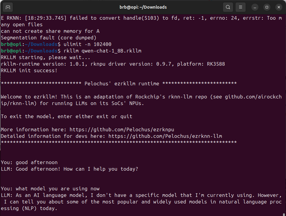
| 22:00, 25 December 2024 | Opi-llm2.png (file) |  |
70 KB | 1 | |
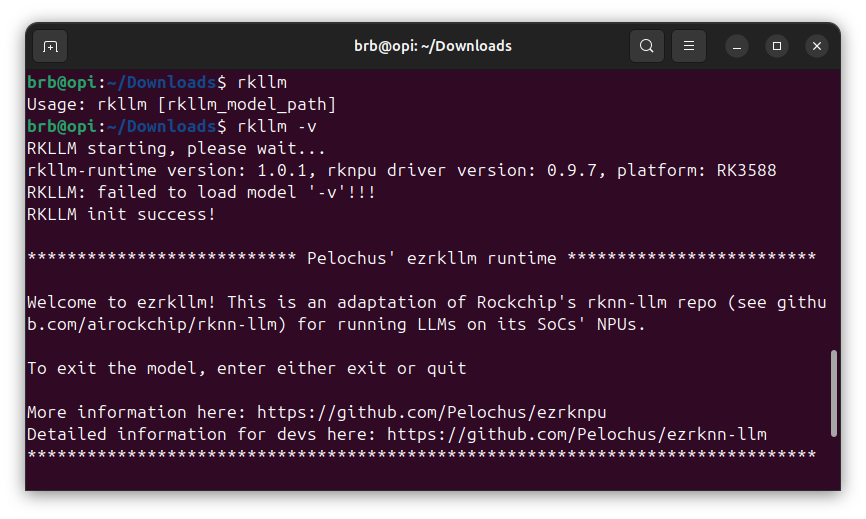
| 22:00, 25 December 2024 | Opi-llm.png (file) |  |
110 KB | 1 | |
| 16:45, 23 December 2024 | Statsheatmapscaled.png (file) |  |
55 KB | 1 | |
| 15:58, 23 December 2024 | Hmx.png (file) |  |
60 KB | 1 | |
| 22:05, 21 December 2024 | Rscales2.png (file) |  |
11 KB | 1 | |
| 22:02, 21 December 2024 | Rscales.svg (file) |  |
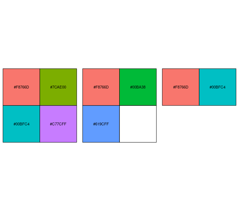
5 KB | <pre> svglite("~/Downloads/Rscales2.svg", bg = "transparent") par(mfrow = c(1, 3),mar = c(0, 4, 0, 2)) show_col(hue_pal()(4)) show_col(hue_pal()(3)) show_col(hue_pal()(2)) par(mfrow = c(1, 1)) dev.off() </pre> | 1 |
| 20:06, 24 August 2024 | R-squared.png (file) |  |
14 KB | 1 | |
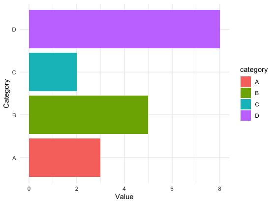
| 14:54, 13 August 2024 | Geom bar reorder.png (file) |  |
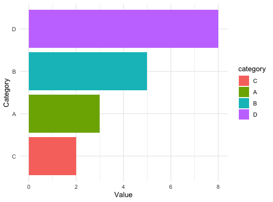
15 KB | <syntaxhighlight lang='r'> library(ggplot2) library(forcats) data <- data.frame( category = c("A", "B", "C", "D"), value = c(3, 5, 2, 8) ) data$category <- fct_reorder(data$category, data$value) levels(data$category) # [1] "C" "A" "B" "D" ggplot(data, aes(x = category, y = value, fill = category)) + geom_bar(stat = "identity") + coord_flip() + labs(x = "Category", y = "Value") + theme_minimal() </syntaxhighlight> | 1 |
| 14:47, 13 August 2024 | Geom bar simple.png (file) |  |
15 KB | <syntaxhighlight lang='r'> library(ggplot2) data <- data.frame( category = c("A", "B", "C", "D"), value = c(3, 5, 2, 8) ) ggplot(data, aes(x = category, y = value, fill = category)) + geom_bar(stat = "identity") + coord_flip() + labs(x = "Category", y = "Value") + # scale_fill_manual(values = c("A" = "red", "B" = "blue", "C" = "green", "D" = "purple")) theme_minimal() </syntaxhighlight> | 1 |
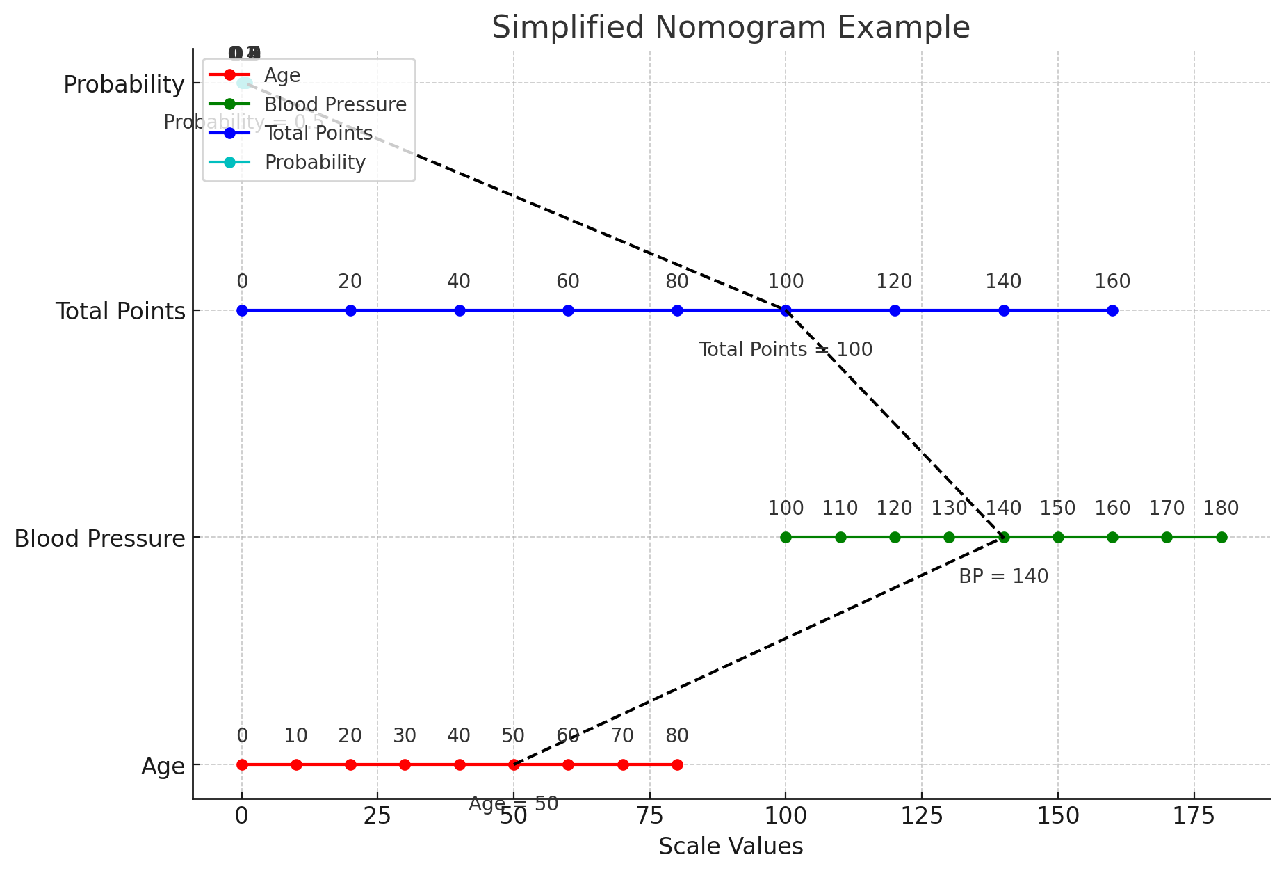
| 12:44, 12 August 2024 | Nomogram.png (file) |  |
145 KB | 1 | |
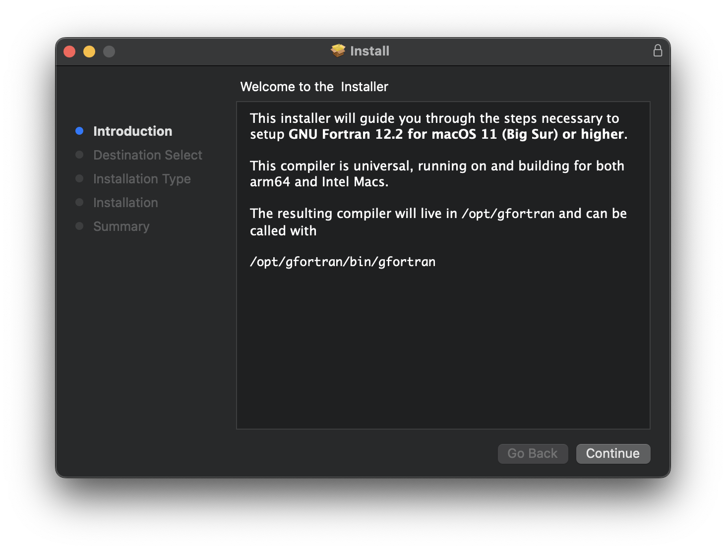
| 14:56, 15 July 2024 | GfortranMac.png (file) |  |
380 KB | 1 | |
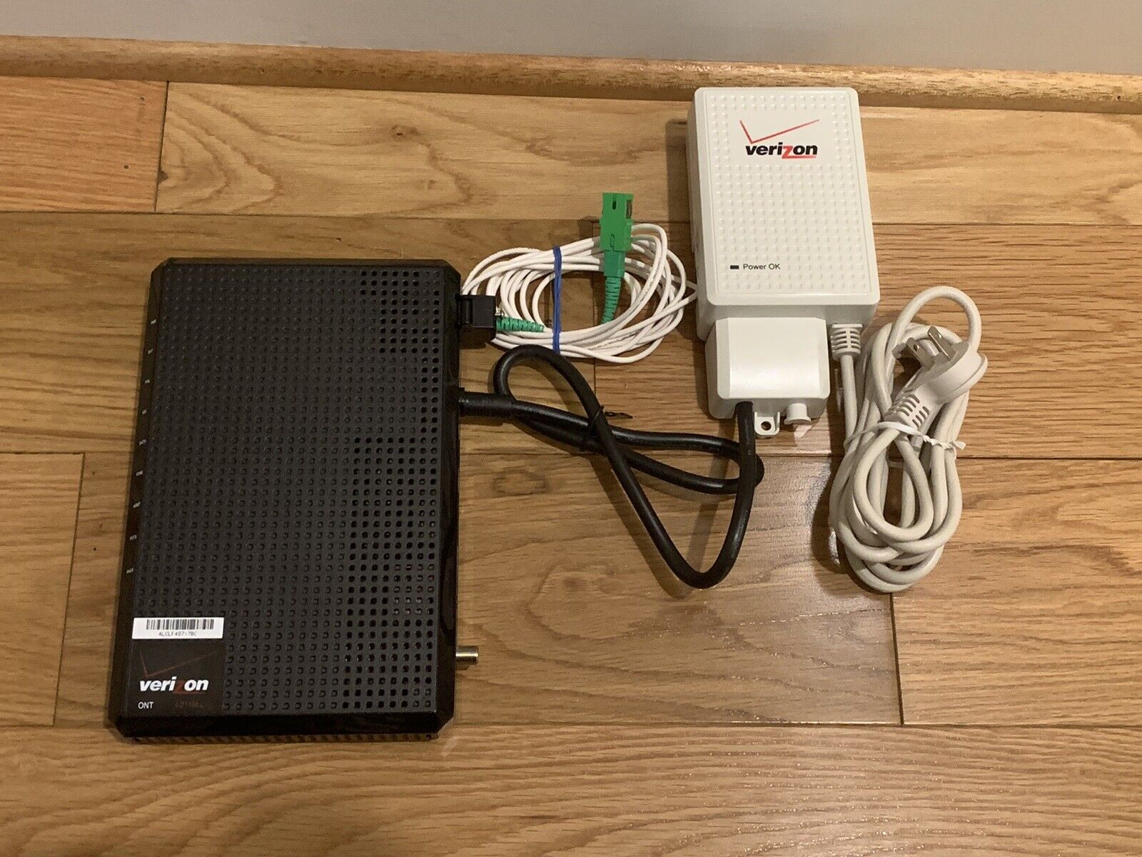
| 07:24, 22 June 2024 | Verizonont.jpg (file) |  |
338 KB | 1 | |
| 12:38, 14 June 2024 | CredoError.png (file) |  |
92 KB | 1 | |
| 13:31, 8 June 2024 | Add camera.png (file) |  |
34 KB | 1 | |
| 14:12, 27 May 2024 | Gganimation.gif (file) |  |
750 KB | <syntaxhighlight lang='r'> library(gganimate) library(ggplot2) library(tidyverse) library(ggimage) data_link <- "https://raw.githubusercontent.com/goodekat/presentations/master/2019-isugg-gganimate-spooky/bat-data/bats-subset.csv" bats <- read.csv(data_link) %>% mutate(id = factor(id)) bat_image_link <- "https://upload.wikimedia.org/wikipedia/en/a/a9/MarioNSMBUDeluxe.png" animation <- bats %>% mutate(image = bat_image_link) %>% filter(id == 1) %>% ggplot(aes(x = longitude, y = la... | 1 |
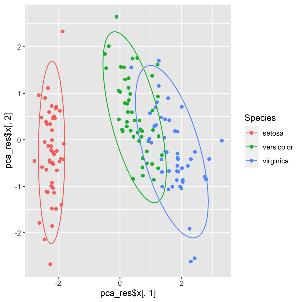
| 08:58, 23 May 2024 | Pca ggplot2.png (file) |  |
136 KB | <syntaxhighlight lang='r'> df <- iris[, 1:4] # exclude "Species" column pca_res <- prcomp(df, scale = TRUE) ggplot(iris, aes(x = pca_res$x[,1], y = pca_res$x[,2], color = Species)) + geom_point() + stat_ellipse() </syntaxhighlight> | 1 |
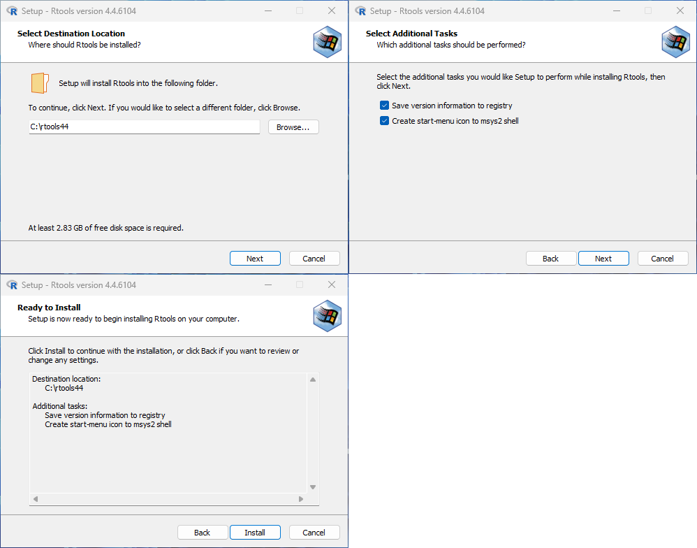
| 14:18, 8 May 2024 | Rtools44.png (file) |  |
57 KB | 1 | |
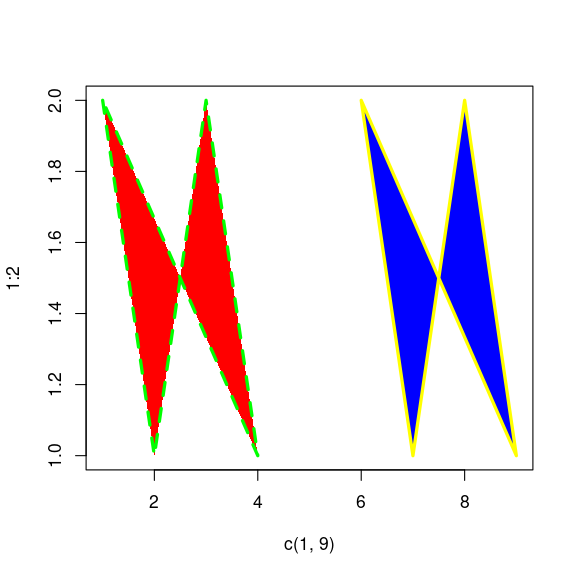
| 16:31, 23 April 2024 | Polygon.png (file) |  |
30 KB | <syntaxhighlight lang='r'> plot(c(1, 9), 1:2, type = "n") polygon(1:9, c(2,1,2,1,NA,2,1,2,1), col = c("red", "blue"), border = c("green", "yellow"), lwd = 3, lty = c("dashed", "solid")) </syntaxhighlight> | 1 |
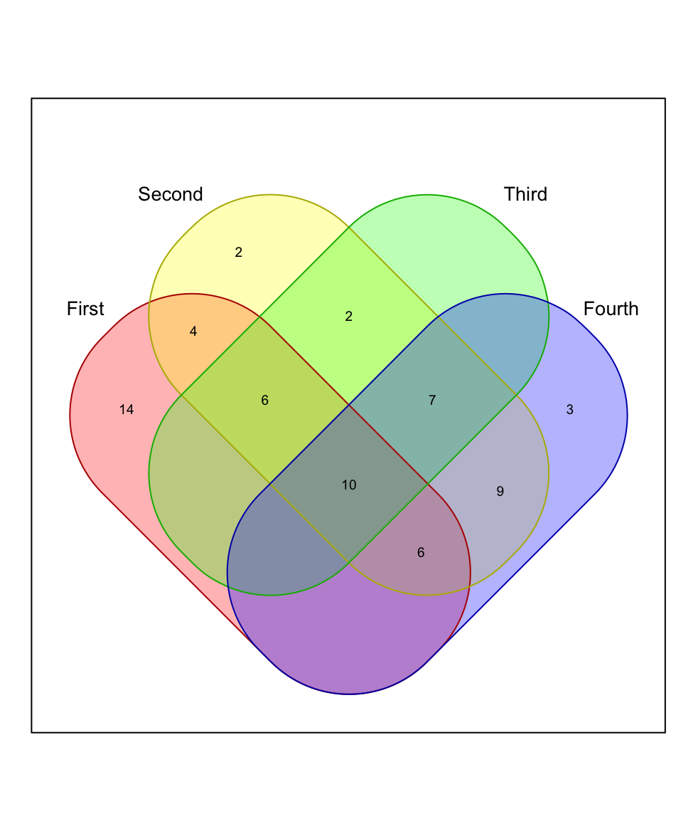
| 13:49, 23 April 2024 | Venn4.png (file) |  |
103 KB | <syntaxhighlight lang='r'> library(venn) set.seed(12345) x <- list(First = 1:40, Second = 15:60, Third = sample(25:50, 25), Fourth=sample(15:65, 35)) venn(x, ilabels = "counts", zcolor = "style") </syntaxhighlight> | 1 |
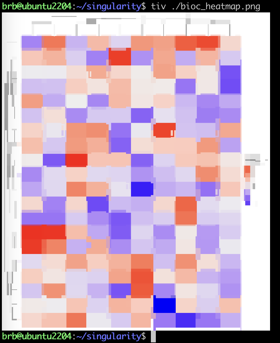
| 14:53, 17 April 2024 | Tiv-demo.png (file) |  |
100 KB | 1 | |
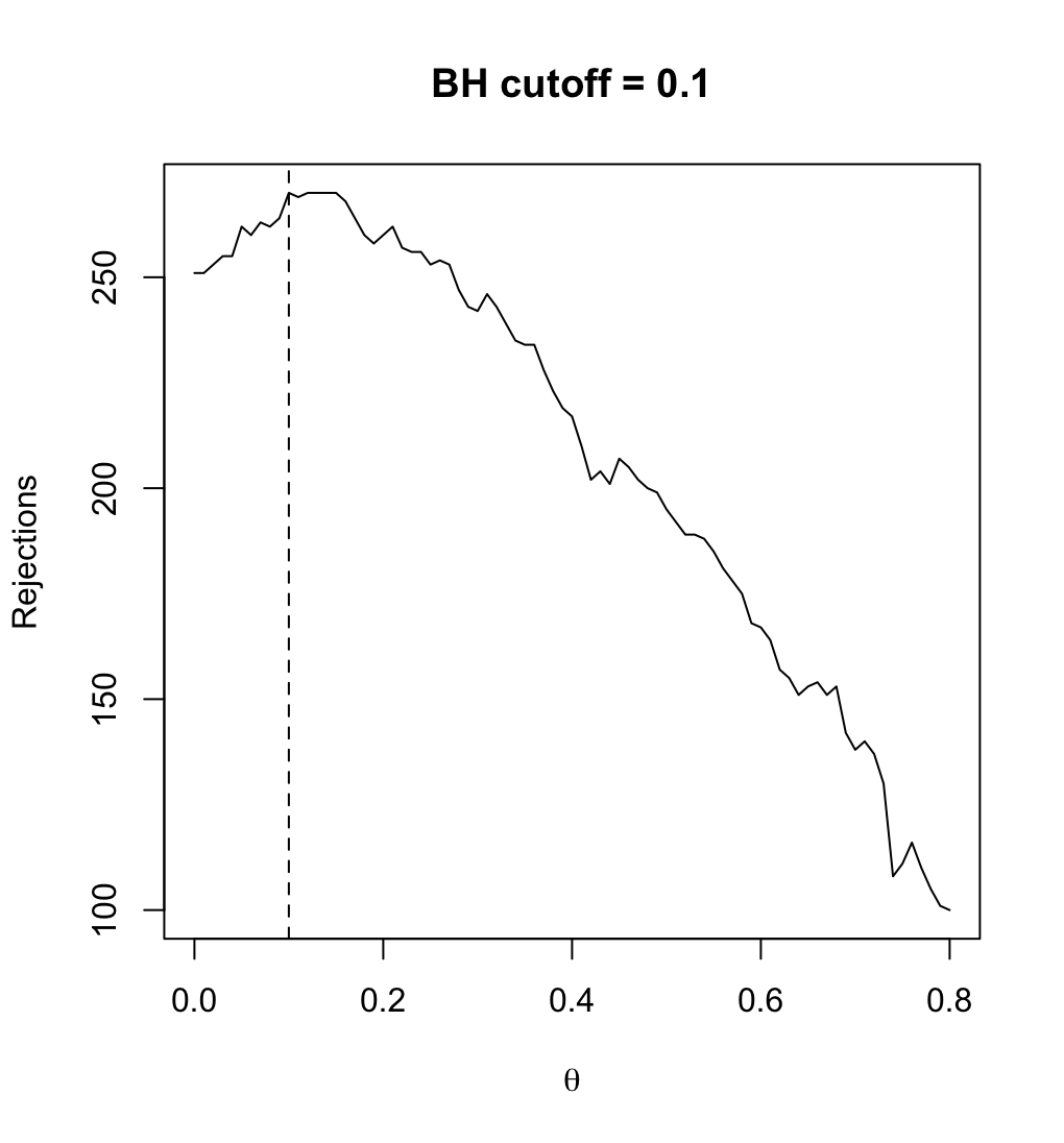
| 19:17, 12 March 2024 | Filtered R mean.png (file) |  |
68 KB | Use sample mean instead of variance for each gene as the filter statistic. <syntaxhighlight lang='r'> # Follow the previous code chunks M2 <- rowMeans(exprs(ALL_bcrneg)) theta <- seq(0, .80, .01) R_BH <- filtered_R(alpha=.10, M2, p2, theta, method="BH") which.max(R_BH) # 10% <---- so theta=0.1 is the optimal; only 10% genes are removed # 11 max(R_BH) # [1] 270 plot(theta, R_BH, type="l", xlab=expression(theta), ylab="Rejections", main="BH cutoff = 0.1") abline(v=.1, lty=2) <... | 1 |
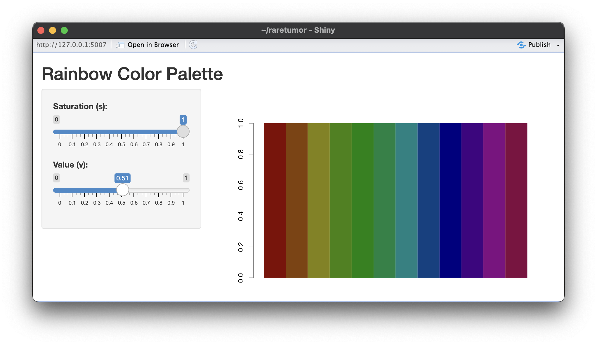
| 07:54, 12 March 2024 | Rainbow v05.png (file) |  |
428 KB | 1 | |
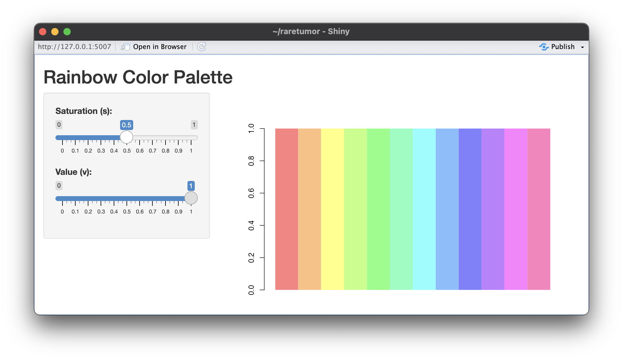
| 07:53, 12 March 2024 | Rainbow s05.png (file) |  |
428 KB | 1 |