Uploads by Brb
Jump to navigation
Jump to search
This special page shows all uploaded files.
| Date | Name | Thumbnail | Size | Description | Versions |
|---|---|---|---|---|---|
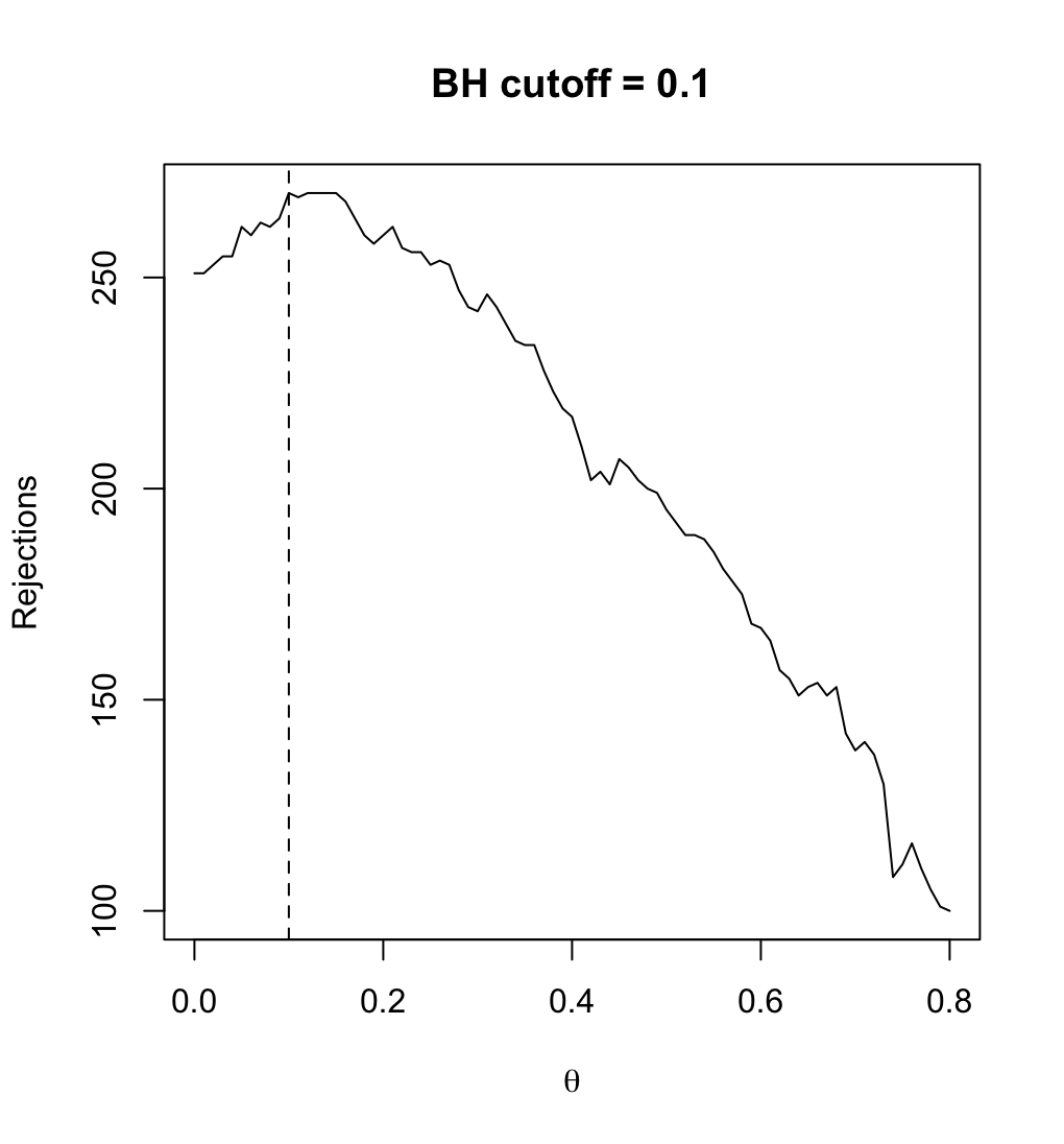
| 20:17, 12 March 2024 | Filtered R mean.png (file) |  |
68 KB | Use sample mean instead of variance for each gene as the filter statistic. <syntaxhighlight lang='r'> # Follow the previous code chunks M2 <- rowMeans(exprs(ALL_bcrneg)) theta <- seq(0, .80, .01) R_BH <- filtered_R(alpha=.10, M2, p2, theta, method="BH") which.max(R_BH) # 10% <---- so theta=0.1 is the optimal; only 10% genes are removed # 11 max(R_BH) # [1] 270 plot(theta, R_BH, type="l", xlab=expression(theta), ylab="Rejections", main="BH cutoff = 0.1") abline(v=.1, lty=2) <... | 1 |
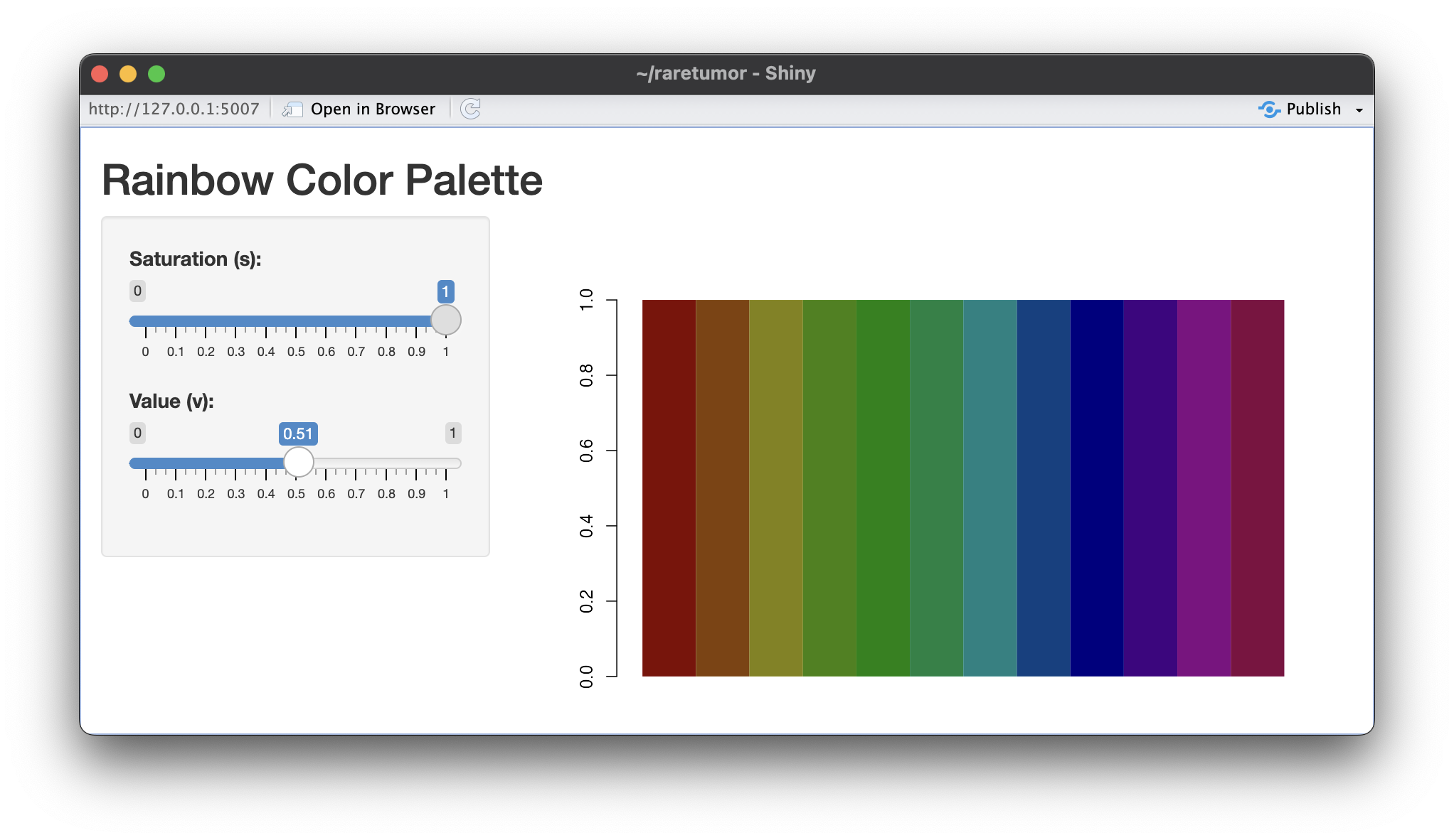
| 08:54, 12 March 2024 | Rainbow v05.png (file) |  |
428 KB | 1 | |
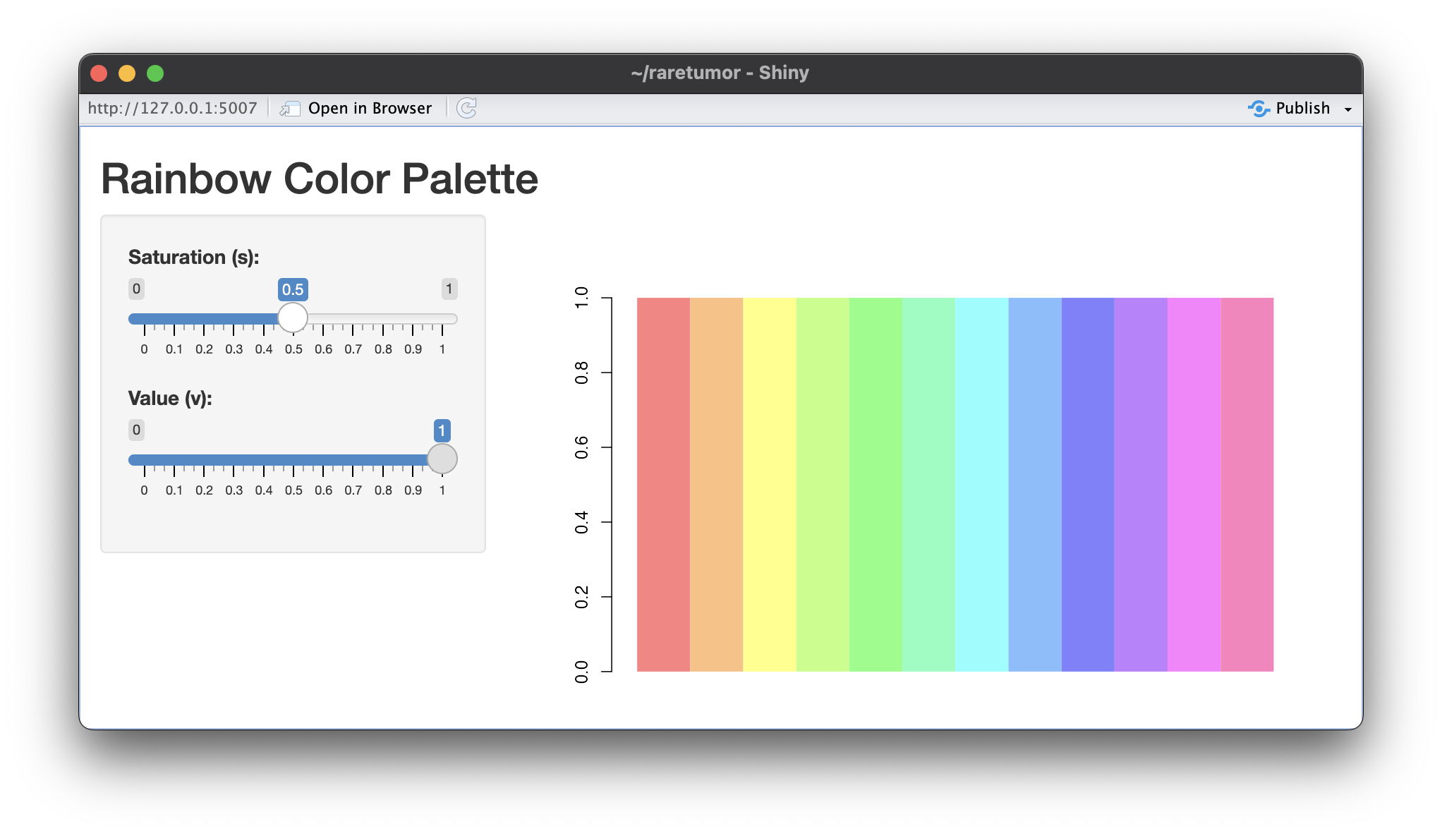
| 08:53, 12 March 2024 | Rainbow s05.png (file) |  |
428 KB | 1 | |
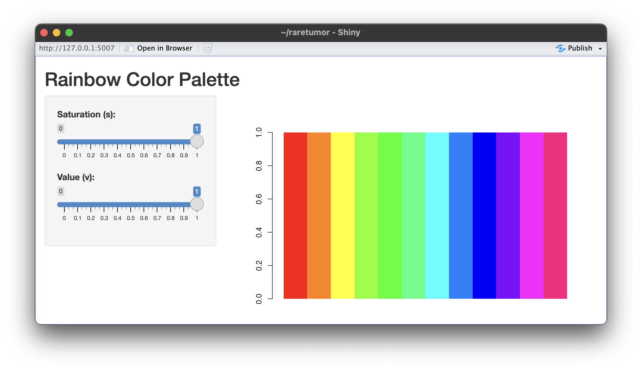
| 08:52, 12 March 2024 | Rainbow default.png (file) |  |
426 KB | <syntaxhighlight lang='r'> library(shiny) # Define the UI ui <- fluidPage( titlePanel("Rainbow Color Palette"), sidebarLayout( sidebarPanel( sliderInput("s_value", "Saturation (s):", min = 0, max = 1, value = 1, step = 0.01), sliderInput("v_value", "Value (v):", min = 0, max = 1, value = 1, step = 0.01) ), mainPanel( plotOutput("rainbow_plot") ) ) ) # Define the server server <- function(input, output) { output$rainbow_plot <- renderPlot({ s <-... | 1 |
| 21:41, 11 March 2024 | Filtered R.png (file) |  |
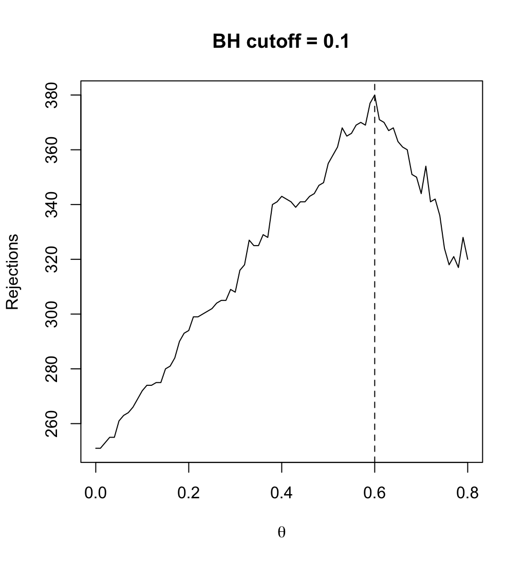
77 KB | <syntaxhighlight lang='r'> theta <- seq(0, .80, .01) R_BH <- filtered_R(alpha=.10, S2, p2, theta, method="BH") which.max(R_BH) # 60% <---- so theta=0.6 is the optimal filtering threshold # 61 max(R_BH) # [1] 380 plot(theta, R_BH, type="l", xlab=expression(theta), ylab="Rejections", main="BH cutoff = 0.1") abline(v=.6, lty=2) </syntaxhighlight> | 1 |
| 21:35, 11 March 2024 | Filtered p.png (file) |  |
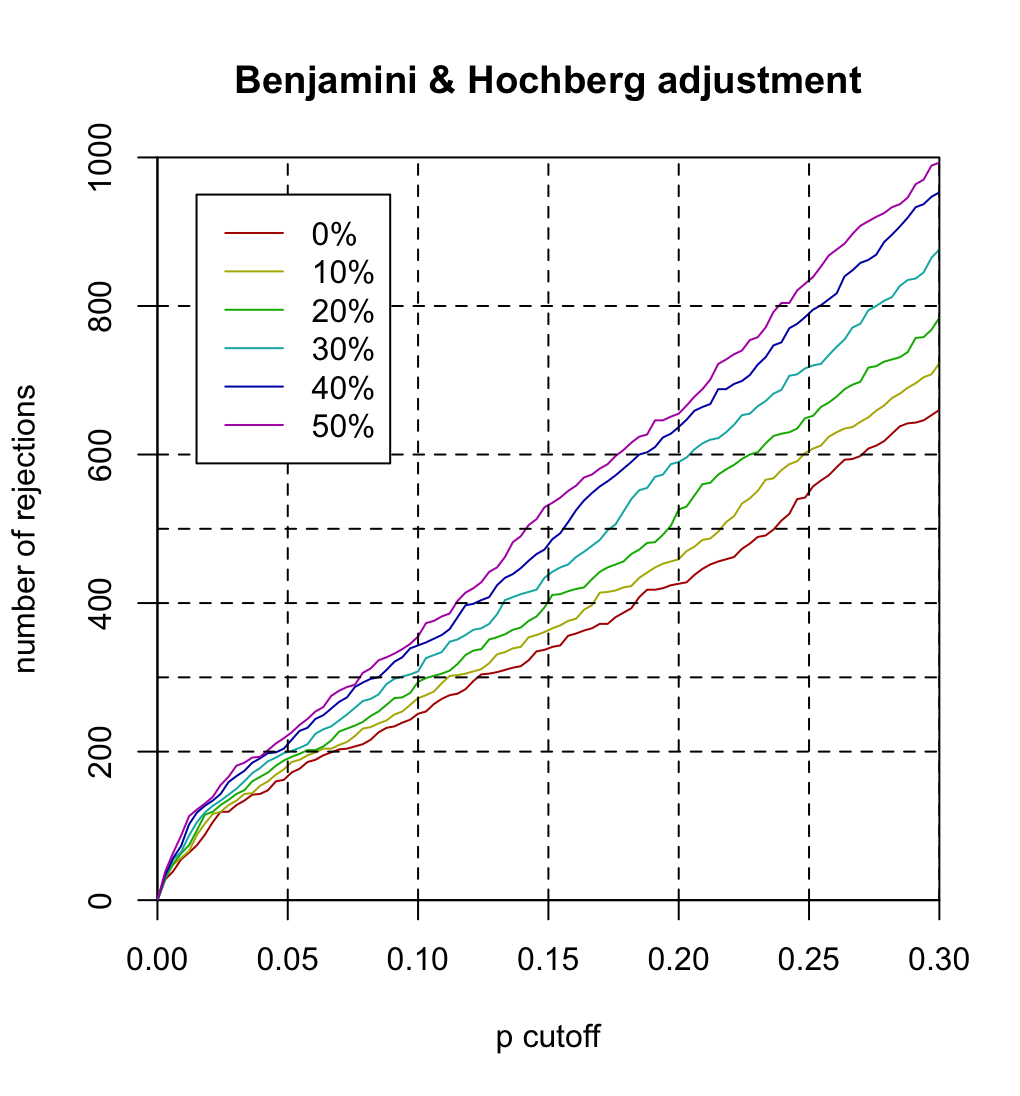
171 KB | Note: # x-axis "p cutoff" should be "BH cutoff" or "FDR cutoff". # Each curve represents theta (filtering threshold). For example, theta=.1 means 10% of genes are filtered out before we do multiple testing (or BH adjustment). # It is seen the larger the theta, the more hypotheses are rejected at the same FDR cutoff. For example, #* if theta=0, 251 hypotheses are rejected at FDR=.1 #* if theta=.5, 355 hypotheses are rejected at FDR=.1. <syntaxhighlight lang='r'> BiocManager::install("ALL")... | 1 |
| 16:49, 8 March 2024 | DataOutliers2.png (file) |  |
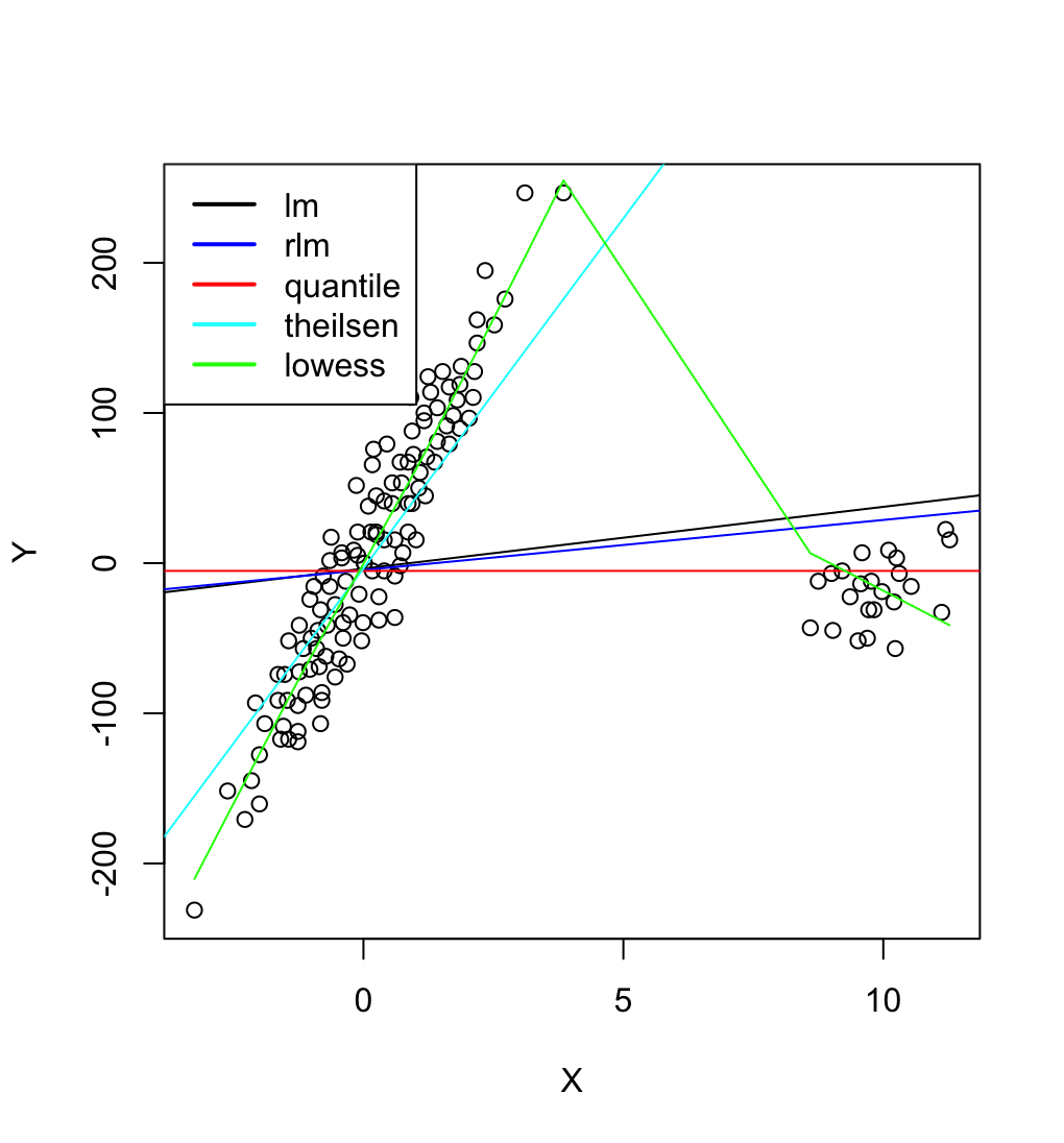
133 KB | {{Pre}} puree <- read.csv("https://gist.githubusercontent.com/arraytools/e851ed88c7456779557fbf3ed67b157a/raw/9971c61fea1db99acbd9de17ea82679ba9811358/dataOutliers2.csv", header=F) plot(puree[,1], puree[, 2], xlab="X", ylab="Y") abline(lm(V2 ~ V1, data = puree)) # robust regression require(MASS) summary(rlm(V2 ~ V1, data = puree)) abline(rr.huber <- rlm(V2 ~ V1, data = puree), col = "blue") # quantile regression library(quantreg) abline(rq(V2 ~ V1, data=puree, tau = 0.5), col = "red") # theil... | 1 |
| 15:27, 7 March 2024 | DataOutliers.png (file) |  |
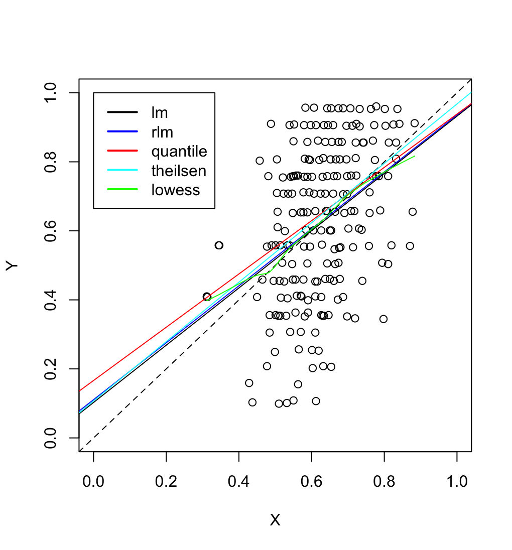
172 KB | {{Pre}} puree <- read.csv("https://gist.githubusercontent.com/arraytools/47d3a46ae1f9a9cd47db350ae2bd2338/raw/b5cccc8e566ff3bef81b1b371e8bfa174c98ef38/dataOutliers.csv", header = FALSE) plot(puree[,1], puree[, 2], xlim=c(0,1), ylim=c(0,1), xlab="X", ylab="Y") abline(0,1, lty=2) abline(lm(V2 ~ V1, data = puree)) # robust regression require(MASS) summary(rlm(V2 ~ V1, data = puree)) abline(rr.huber <- rlm(V2 ~ V1, data = puree), col = "blue") # almost overlapped with lm() # quantile regressio... | 1 |
| 22:41, 10 February 2024 | R162.png (file) |  |
25 KB | 1 | |
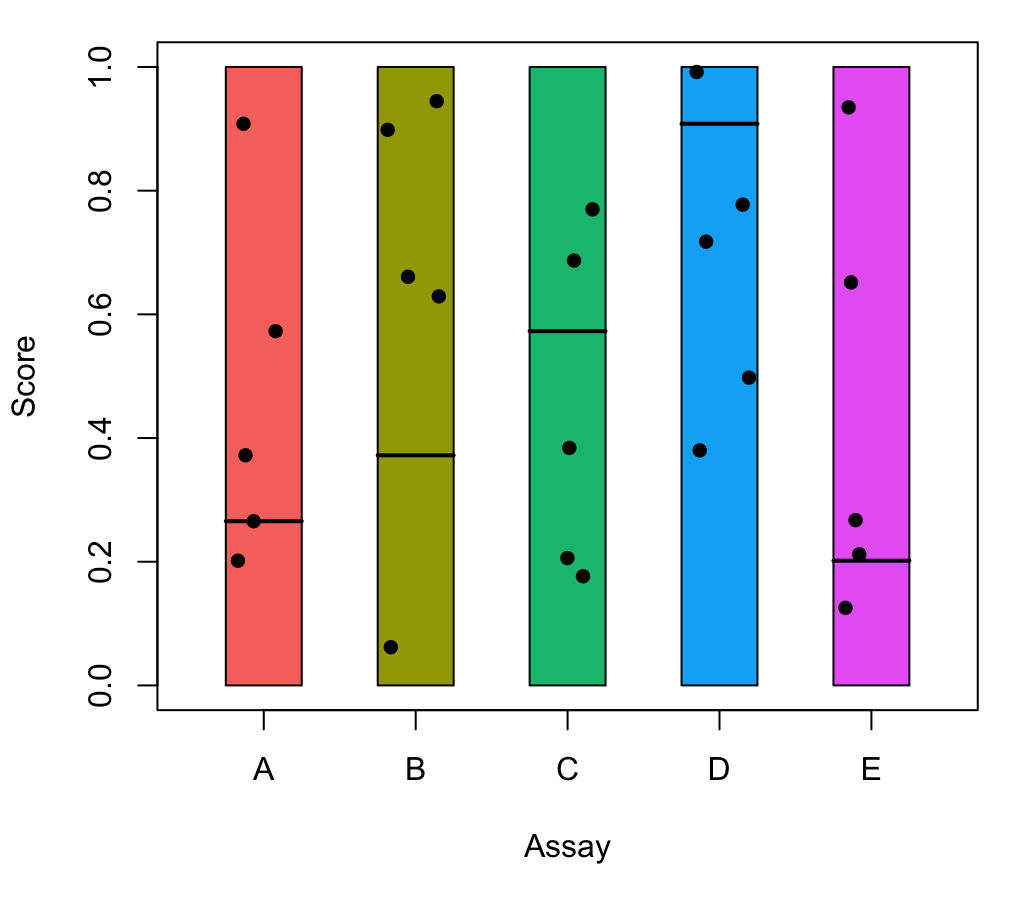
| 22:53, 8 February 2024 | Jitterbox.png (file) |  |
50 KB | <syntaxhighlight lang='r'> nc <- 5 assy <- LETTERS[1:nc] pal <- ggpubr::get_palette("default", nc) set.seed(1) nr <- 5 mat <- matrix(runif(nr*length(assy)), nrow = nr, ncol = length(assy)) set.seed(1) cutoffs <- runif(nc) colnames(mat) <- assy par(mar=c(5,4,1,1)+.1) plot(1, 1, xlim = c(0.5, nc + .5), ylim = c(0,1), type = "n", xlab = "Assay", ylab = "Score", xaxt = 'n') for (i in 1:nc) { rect(i - 0.25, 0, i + 0.25, 1, col = pal[i]) lines(x = c(i - 0.25, i + 0.25), y = c(cutof... | 1 |
| 11:25, 19 January 2024 | RStudioAbort.png (file) |  |
38 KB | 1 | |
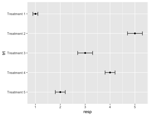
| 20:38, 15 October 2023 | Geomerrorbarh.png (file) |  |
17 KB | <syntaxhighlight lang='rsplus'> df <- data.frame( trt = factor(c("Treatment 1", "Treatment 2", "Treatment 3", "Treatment 4", "Treatment 5")), # treatment resp = c(1, 5, 3, 4, 2), # response se = c(0.1, 0.3, 0.3, 0.2, 0.2) # standard error ) # make 'Treatment 1' shown at the top df$trt <- factor(df$trt, levels = c("Treatment 5", "Treatment 4", "Treatment 3", "Treatment 2", "Treatment 1")) p <- ggplot(df, aes(resp, trt)) + geom_point() p + geom_errorbarh(aes(xmax=resp + se, xmin=resp-se),... | 1 |
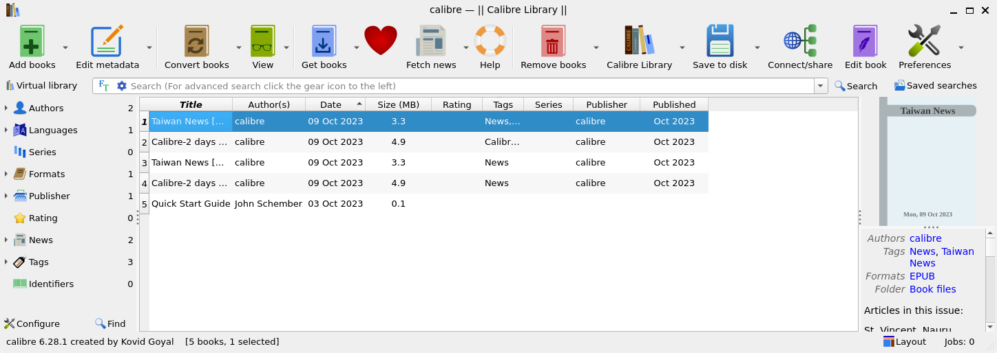
| 17:32, 9 October 2023 | Calibre.png (file) |  |
128 KB | 1 | |
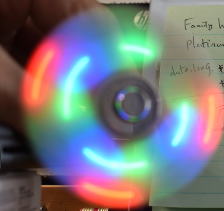
| 12:18, 24 August 2023 | Wheel f400.png (file) |  |
200 KB | 1 | |
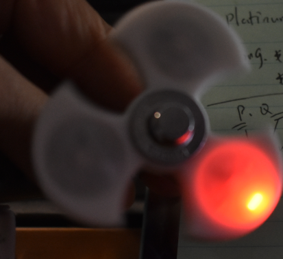
| 12:17, 24 August 2023 | Wheel f8.png (file) |  |
224 KB | 1 | |
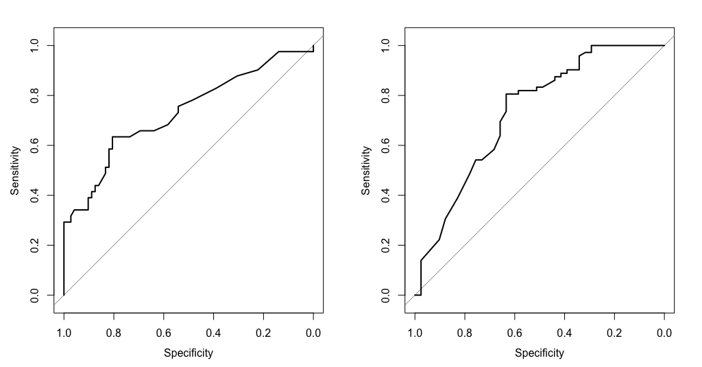
| 15:59, 22 August 2023 | Roc asah.png (file) |  |
38 KB | <pre> par(mfrow=c(1,2)) roc(aSAH$outcome, aSAH$s100b, plot = T) roc(aSAH$outcome2, aSAH$s100b, plot = T) par(mfrow=c(1,1)) </pre> | 1 |
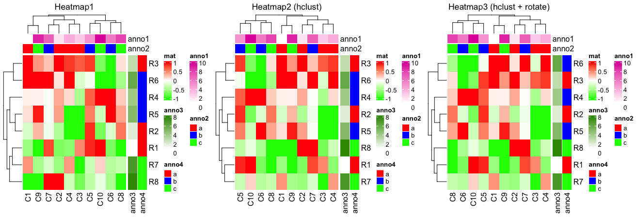
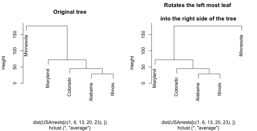
| 14:44, 13 August 2023 | Rotateheatmap.png (file) |  |
52 KB | <syntaxhighlight lang="rsplus"> library(circlize) set.seed(123) mat = matrix(rnorm(80), 8, 10) rownames(mat) = paste0("R", 1:8) colnames(mat) = paste0("C", 1:10) col_anno = HeatmapAnnotation( df = data.frame(anno1 = 1:10, anno2 = rep(letters[1:3], c(4,3,3))), col = list(anno2 = c("a" = "red", "b" = "blue", "c" = "green"))) row_anno = rowAnnotation( df = data.frame(anno3 = 1:8, anno4 = rep(l... | 1 |
| 16:21, 12 August 2023 | Rotatedend.png (file) |  |
17 KB | 1 | |
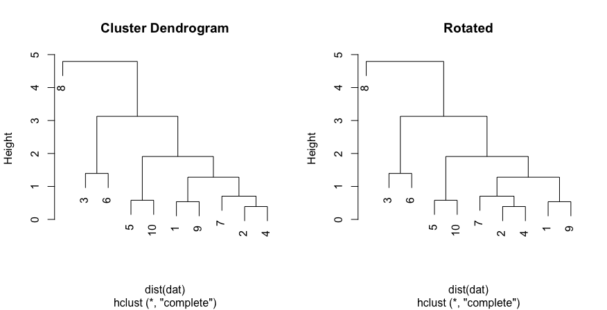
| 16:17, 12 August 2023 | Dend12.png (file) |  |
11 KB | {{Pre}} set.seed(123) dat <- matrix(rnorm(20), ncol=2) # perform hierarchical clustering hc <- hclust(dist(dat)) # plot dendrogram plot(hc) # get ordering of leaves ord <- order.dendrogram(as.dendrogram(hc)) ord # [1] 8 3 6 5 10 1 9 7 2 4 # Same as seen on the dendrogram nodes # Rotate the branches (1,9) & (7,2,4) plot(rotate(hc, c("8", "3", "6", "5", "10", "7", "2", "4", "1", "9")), main="Rotated") </pre> | 1 |
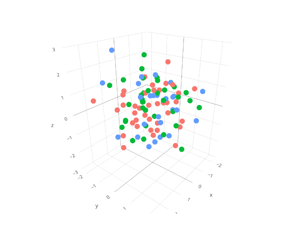
| 16:39, 6 August 2023 | Plotly3d.png (file) |  |
90 KB | 1 | |
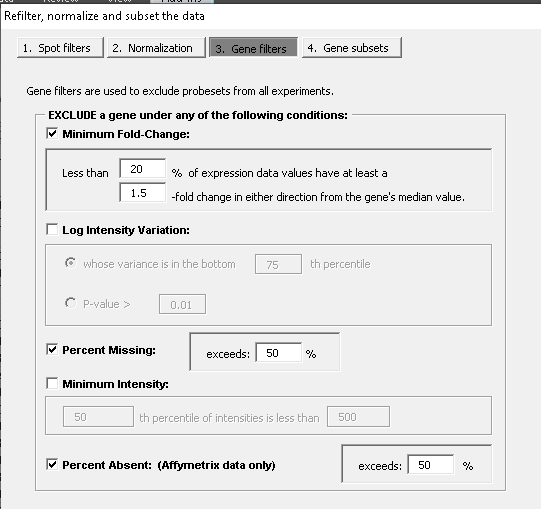
| 15:39, 31 July 2023 | Filter single.png (file) |  |
15 KB | 1 | |
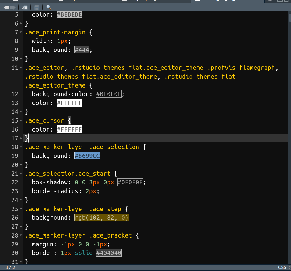
| 12:47, 27 May 2023 | Vibrant ink rstheme.png (file) |  |
115 KB | https://github.com/captaincaed/rstudio/blob/main/vibrant_ink_SB_2.rstheme | 1 |
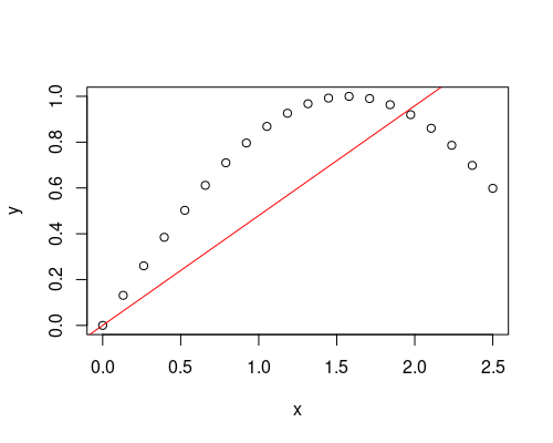
| 13:46, 21 May 2023 | R2.png (file) |  |
15 KB | <syntaxhighlight lang='rsplus'> x <- seq(0, 2.5, length=20) y <- sin(x) plot(x, y) abline(lsfit(x, y, intercept = F), col = 'red') summary(fit)$r.squared # [1] 0.8554949 </syntaxhighlight> | 1 |
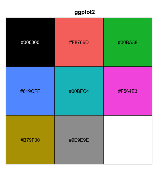
| 16:02, 11 May 2023 | Paletteggplot2.png (file) |  |
25 KB | 1 | |
| 12:12, 10 May 2023 | Paletteshowcol.png (file) |  |
24 KB | 1 | |
| 11:15, 10 May 2023 | Palettebarplot.png (file) |  |
9 KB | <syntaxhighlight lang='rsplus'> pal <- c("#E41A1C", "#377EB8", "#4DAF4A", "#984EA3", "#FF7F00") # pal <- sample(colors(), 10) # randomly pick 10 colors barplot(rep(1, length(pal)), col = pal, space = 0, axes = FALSE, border = NA) </syntaxhighlight> | 1 |
| 11:14, 10 May 2023 | Paletteheatmap.png (file) |  |
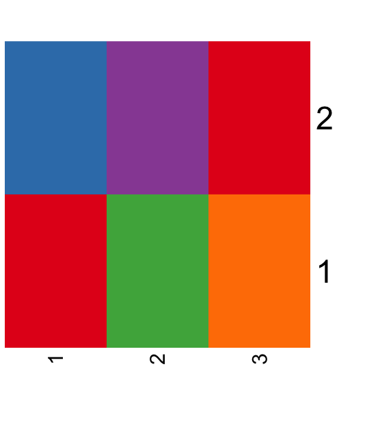
12 KB | <syntaxhighlight lang='rsplus'> pal <- c("#E41A1C", "#377EB8", "#4DAF4A", "#984EA3", "#FF7F00") pal <- matrix(pal, nr=2) # acknowledge a nice warning message pal_matrix <- matrix(seq_along(pal), nr=nrow(pal), nc=ncol(pal)) heatmap(pal_matrix, col = pal, Rowv = NA, Colv = NA, scale = "none", ylab = "", xlab = "", main = "", margins = c(5, 5)) # 2 rows, 3 columns with labeling on two axes </syntaxhighlight> | 1 |
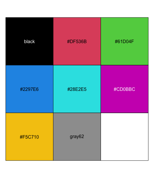
| 11:08, 10 May 2023 | Rpalette.png (file) |  |
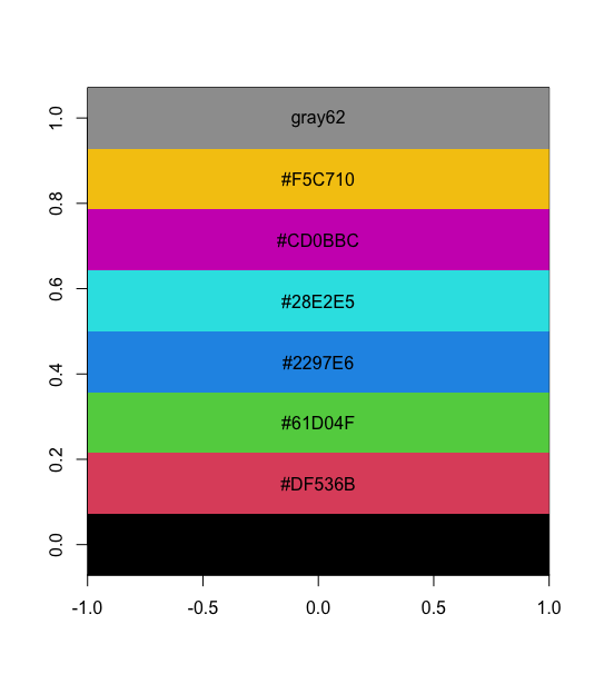
28 KB | <syntaxhighlight lang='rsplus'> pal <- palette() # [1] "black" "#DF536B" "#61D04F" "#2297E6" "#28E2E5" "#CD0BBC" "#F5C710" # [8] "gray62" pal_matrix <- matrix(seq_along(pal), nr=1) image(pal_matrix, col = pal, axes = FALSE) # 8 rows, 1 column, but no labeling # Starting from bottom, left. par()$usr # change with the data dim text(0, (par()$usr[4]-par()$usr[3])/8*c(0:7), labels = pal) </syntaxhighlight> | 1 |
| 13:52, 9 May 2023 | Ggplotbarplot.png (file) |  |
23 KB | 1 | |
| 11:40, 9 May 2023 | Cbioportal cptac.png (file) |  |
120 KB | 1 | |
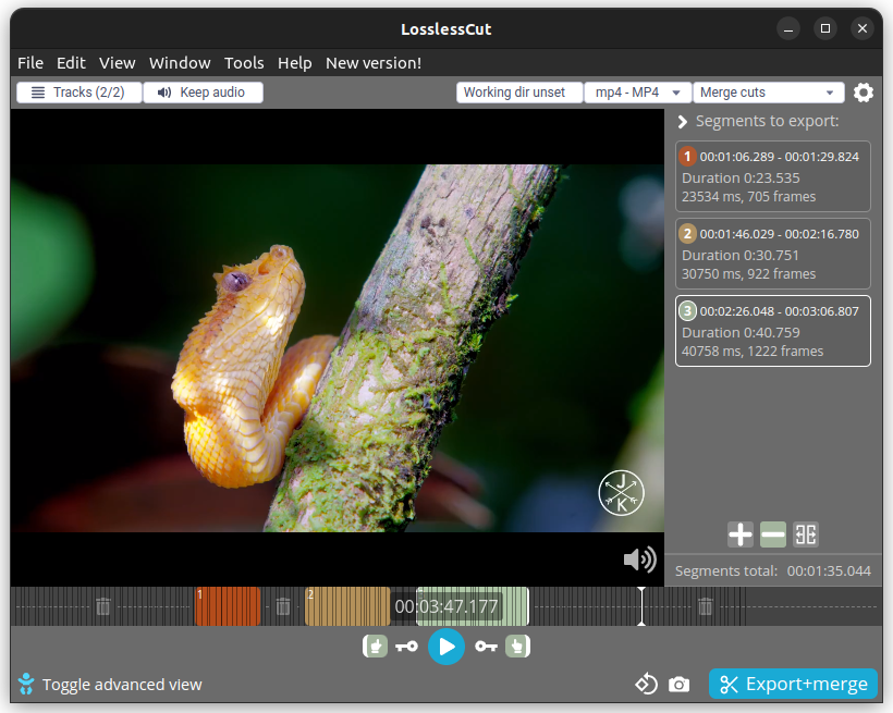
| 21:07, 25 April 2023 | Losslesscut.png (file) |  |
323 KB | 1 | |
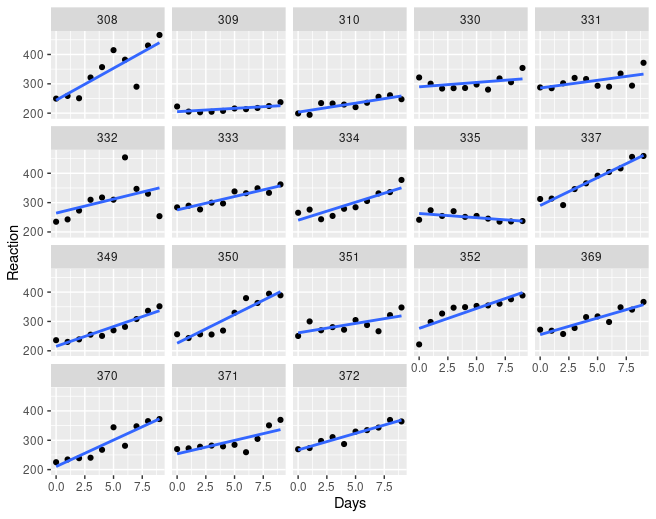
| 17:47, 23 April 2023 | Sleepstudy.png (file) |  |
59 KB | <syntaxhighlight lang='rsplus'> sleepstudy %>% ggplot(aes(x=Days, y = Reaction)) + geom_point() + geom_smooth(method = "lm", se = FALSE) + facet_wrap(~Subject) </syntaxhighlight> | 1 |
| 16:58, 17 March 2023 | Svg4.svg (file) |  |
33 KB | <pre> svg("svg4.svg", width=4, height=4) plot(1:10, main="width=4, height=4") dev.off() </pre> | 1 |
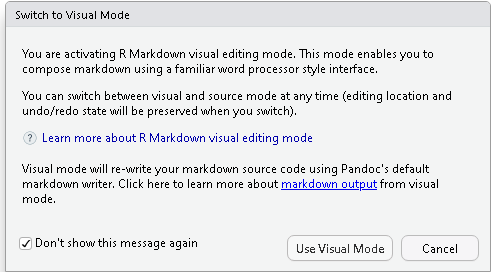
| 10:44, 11 March 2023 | RStudioVisualMode.png (file) |  |
10 KB | 1 | |
| 16:01, 8 March 2023 | Pca directly2.png (file) |  |
35 KB | 1 | |
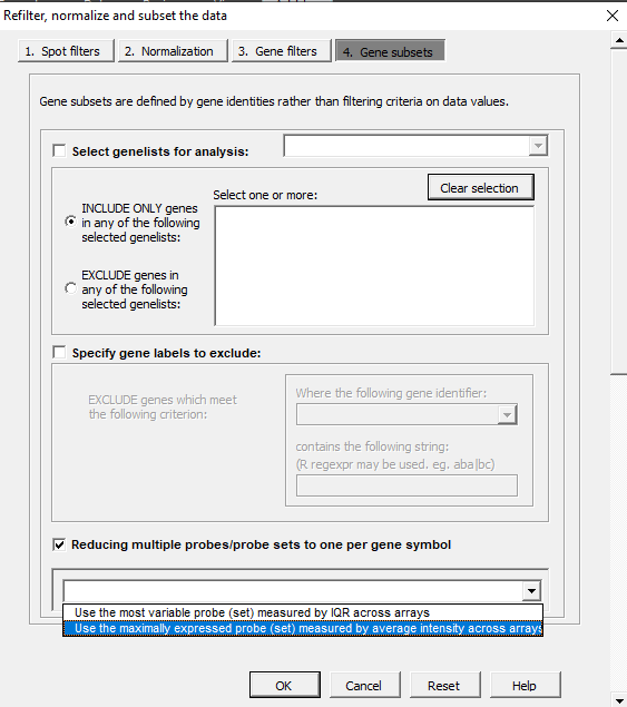
| 11:11, 11 February 2023 | MultipleProbes.PNG (file) |  |
28 KB | 1 | |
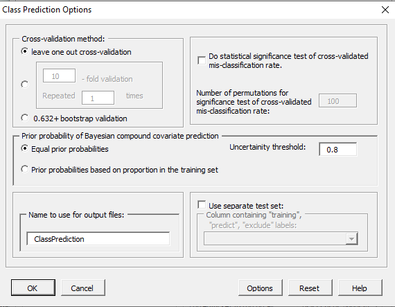
| 11:10, 11 February 2023 | ClassPredictionOptions.PNG (file) |  |
21 KB | 1 | |
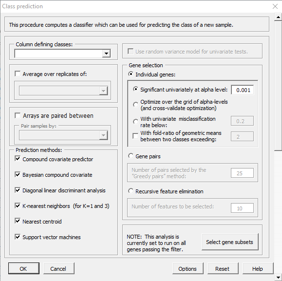
| 11:08, 11 February 2023 | ClassPrediction.PNG (file) |  |
34 KB | 1 | |
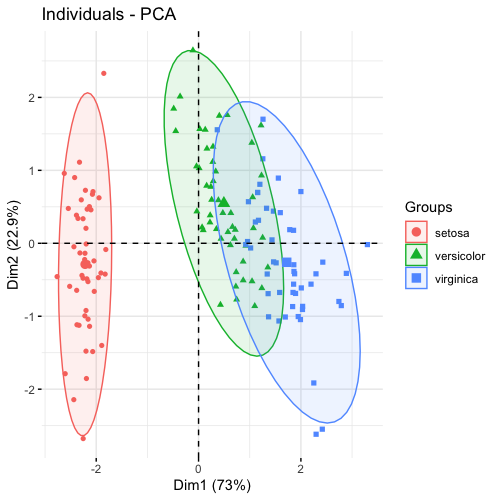
| 21:01, 28 January 2023 | Pca factoextra.png (file) |  |
60 KB | 1 | |
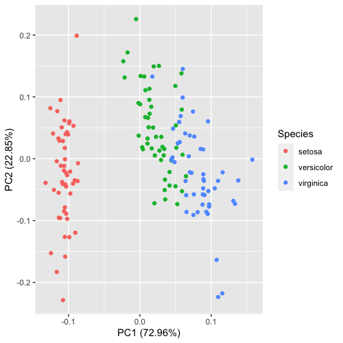
| 20:34, 28 January 2023 | Pca autoplot.png (file) |  |
41 KB | 1 | |
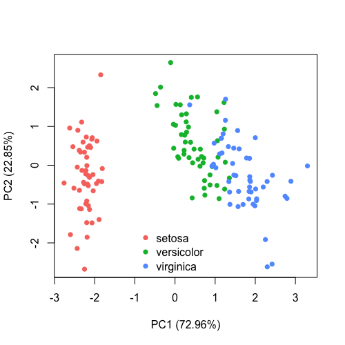
| 20:34, 28 January 2023 | Pca directly.png (file) |  |
40 KB | 1 | |
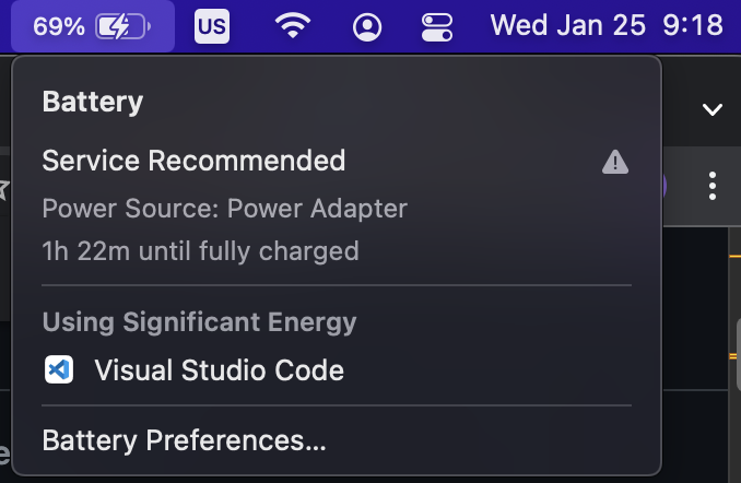
| 10:21, 25 January 2023 | VscodeEnergy.png (file) |  |
116 KB | 1 | |
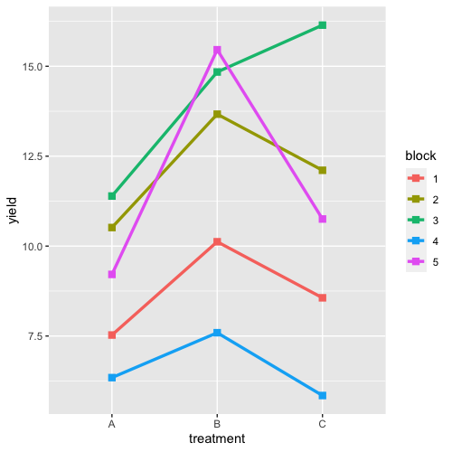
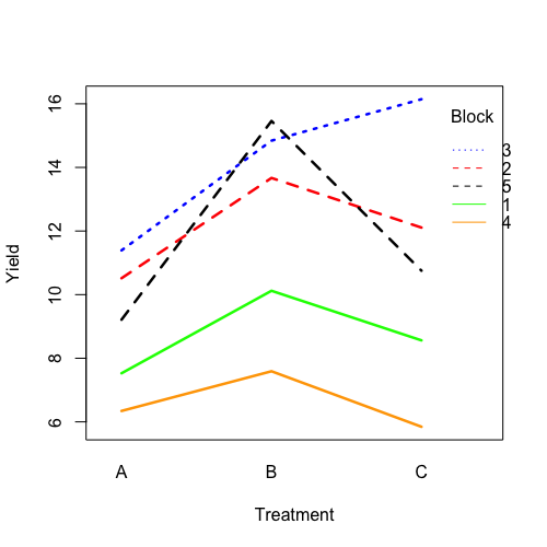
| 22:26, 14 January 2023 | RbdGeom.png (file) |  |
41 KB | <pre> require(ggplot2) aggregate( .~ treatment +block,FUN=median, data = data) |> ggplot(aes(treatment, yield)) + geom_line(aes(group = block, color = block), linewidth = 1.2) + geom_point(aes(color = block), shape = 15, size=2.6) </pre> | 1 |
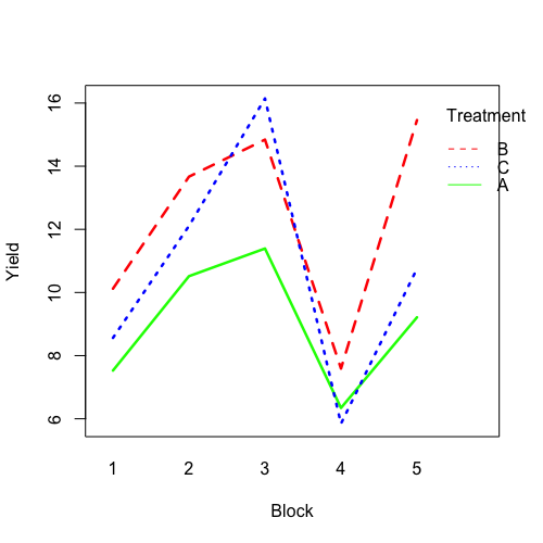
| 21:51, 14 January 2023 | RbdBlock.png (file) |  |
34 KB | <pre> set.seed(1234) block <- as.factor(rep(1:5, each=6)) treatment <- rep(c("A","B","C"),5) block_shift <- rnorm(5, mean = 0, sd = 2) treatment_shift <- c(A=0, B=4, C=2) random_effect <- rnorm(30, mean = 0, sd = 1) yield <- rnorm(30, mean = 10, sd = 2) + treatment_shift[as.integer(factor(treatment))] + block_shift[as.numeric(block)] + random_effect data <- data.frame(block, treatment, yield) summary(fm1 <- aov(yield ~ treatment + block, data = data)) # Df Sum Sq Mean Sq... | 1 |
| 21:50, 14 January 2023 | RbdTreat.png (file) |  |
32 KB | <pre> set.seed(1234) block <- as.factor(rep(1:5, each=6)) treatment <- rep(c("A","B","C"),5) block_shift <- rnorm(5, mean = 0, sd = 2) treatment_shift <- c(A=0, B=4, C=2) random_effect <- rnorm(30, mean = 0, sd = 1) yield <- rnorm(30, mean = 10, sd = 2) + treatment_shift[as.integer(factor(treatment))] + block_shift[as.numeric(block)] + random_effect data <- data.frame(block, treatment, yield) summary(fm1 <- aov(yield ~ treatment + block, data = data)) # Df Sum Sq Mean Sq... | 1 |
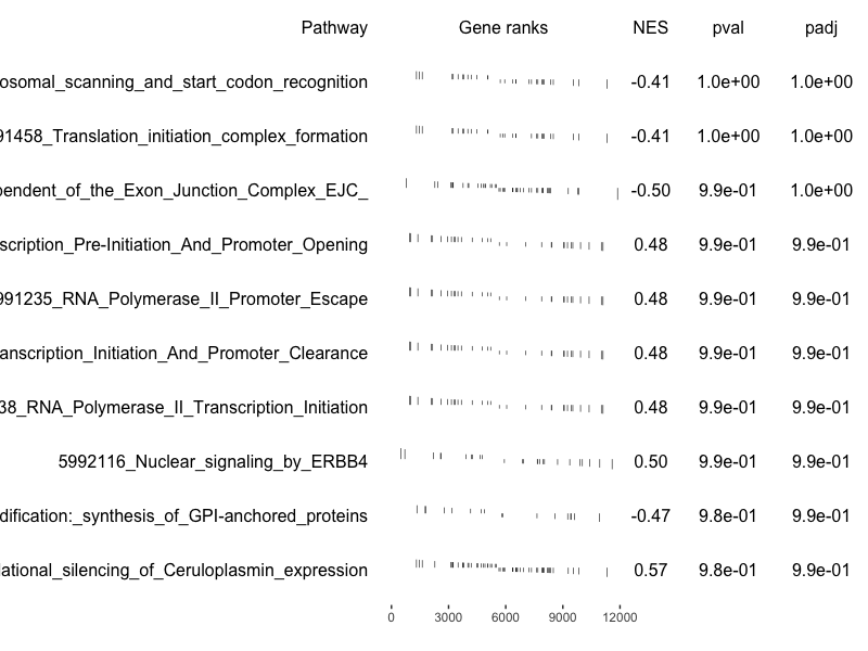
| 12:18, 12 January 2023 | GseaTable2.png (file) |  |
81 KB | An example of a plot from 10 non-enriched pathways. <pre> data(examplePathways) data(exampleRanks) fgseaRes <- fgsea(examplePathways, exampleRanks, nperm=1000, minSize=15, maxSize=100) fgseaRes[order(pval, decreasing = T),][1:10, c('NES', 'pval')] # NES pval # 1: -0.4050950 1.0000000 # 2: -0.4050950 1.0000000 # 3: -0.4966664 0.9932584 # 4: 0.4804114 0.9870610 # 5: 0.4804114 0.9870610 # 6: 0.4804114 0.9870610 # 7: 0.4804114 0.9870610 # 8: 0.4955139 0.9854... | 1 |
| 12:01, 12 January 2023 | GseaTable.png (file) |  |
81 KB | <pre> data(examplePathways) data(exampleRanks) fgseaRes <- fgsea(examplePathways, exampleRanks, nperm=1000, minSize=15, maxSize=100) # I pick 5 pathways with + NES and 5 pathways with - NES. fgseaRes[order(pval), ][62:71, c('pathway', 'NES')] # pathway NES # 1: 5992282_ECM_proteoglycans 1.984081 # 2: 5992219_Regulation_of_cholesterol_biosynthesis_by_SREBP_SREBF_ 1.95... | 1 |
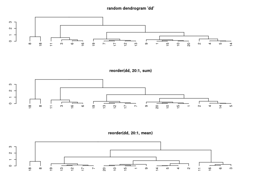
| 12:15, 8 January 2023 | Reorder.dendrogram.png (file) |  |
10 KB | <pre> set.seed(123) x <- rnorm(20) hc <- hclust(dist(x)) dd <- as.dendrogram(hc) par(mfrow=c(3, 1)) plot(dd, main = "random dendrogram 'dd'") # not the same as reorder(dd, 1:20) plot(reorder(dd, 20:1), main = 'reorder(dd, 20:1, sum)') plot(reorder(dd, 20:1, mean), main = 'reorder(dd, 20:1, mean)') </pre> | 1 |
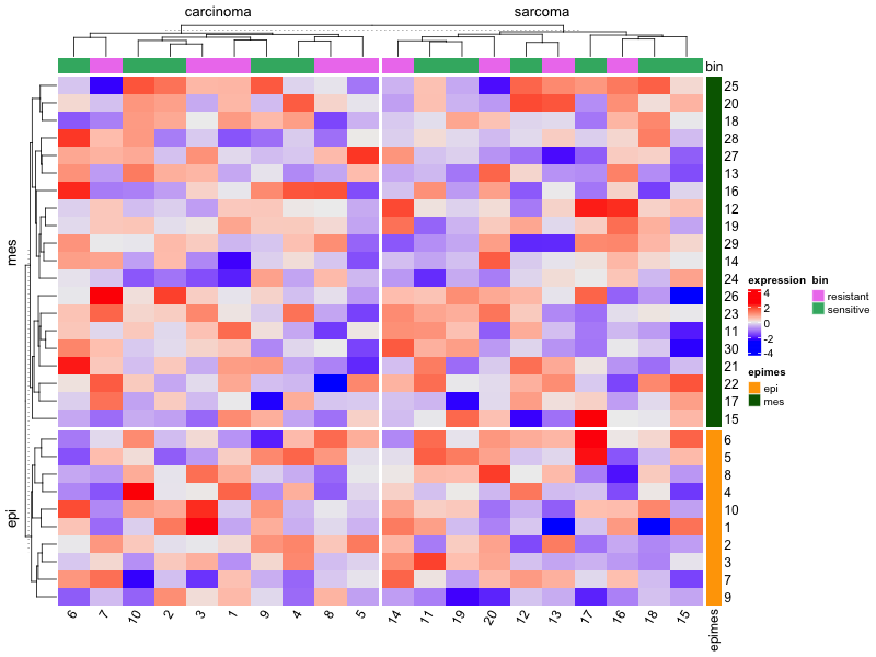
| 21:37, 7 January 2023 | ComplexHeatmap2.png (file) |  |
43 KB | <syntaxhighlight lang="rsplus"> # Simulate data library(ComplexHeatmap) ng <- 30; ns <- 20 set.seed(1) mat <- matrix(rnorm(ng*ns), nr=ng, nc=ns) colnames(mat) <- 1:ns rownames(mat) <- 1:ng # color bar on RHS ind_e <- 1:round(ng/3) ind_m <- (1+round(ng/3)):ng epimes <- rep(c("epi", "mes"), c(length(ind_e), length(ind_m))) row_ha <- rowAnnotation(epimes = epimes, col = list(epimes = c("epi" = "orange", "mes" = "darkgreen"))) # color bar on Top tumortype <- rep(c("carcinoma", "sarcoma"... | 1 |
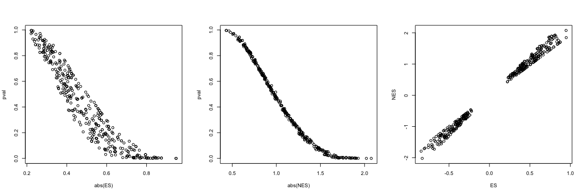
| 12:37, 6 January 2023 | Fgsea3plots.png (file) |  |
68 KB | <pre> par(mfrow=c(1,3)) with(fgseaRes, plot(abs(ES), pval)) with(fgseaRes, plot(abs(NES), pval)) with(fgseaRes, plot(ES, NES)) </pre> | 1 |