Batch effect

Merging two gene expression studies

Possible batch

STAT115 Chapter 6.5 Batch Effect Removal

ComBat

• Adjusting batch effects in microarray expression data using empirical Bayes methods Johnson 2006. Note the term "ComBat" has not been used.
• Statistics for Genomic Data Science (Coursera) and https://github.com/jtleek/genstats
• Some possible batch variables: operators, runs, machines, library kits, laboratories.
• sva::ComBat() function in sva package from Bioconductor. [math]\displaystyle{ \begin{align} Y_{ijg} = \alpha_g + X \beta_g + \gamma_{ig} + \delta_{ig} \epsilon_{ijg} \end{align} }[/math] where [math]\displaystyle{ X=X_{ij} }[/math] consists of covariates (eg biological) of scientific interests (e.g. Pathway activation levels in Zhang's 2018 simulation example), while [math]\displaystyle{ \gamma_{ig} }[/math] and [math]\displaystyle{ \delta_{ig} }[/math] characterize the additive and multiplicative batch effects of batch i for gene g. The error terms, [math]\displaystyle{ \epsilon_{ijg} }[/math], are assumed to follow a normal distribution with expected value of zero and variance [math]\displaystyle{ \sigma^2_𝑔 }[/math]. The batch corrected data is [math]\displaystyle{ \begin{align} \frac{Y_{ijg} - \hat{\alpha_g} - X \hat{\beta_g} - \hat{\gamma_{ig}}}{\hat{\delta_{ig}}} + \hat{\alpha_g} + X \hat{\beta_g}. \end{align} }[/math]
• Alternative empirical Bayes models for adjusting for batch effects in genomic studies Zhang et al. BMC Bioinformatics 2018. The R package is sva and BatchQC from Bioconductor.
  • Reference batch adjustment: [math]\displaystyle{ \begin{align} Y_{ijg} = \alpha_{rg} + X \beta_{rg} + \gamma_{rig} + \delta_{rig} \epsilon_{ijg} \end{align} }[/math] where [math]\displaystyle{ \alpha_{rg} }[/math] is the average gene expression in the chosen reference batch (r). Furthermore, [math]\displaystyle{ \gamma_{rig} }[/math] and [math]\displaystyle{ \delta_{rig} }[/math] represent the additive and multiplicative batch differences between the reference batch and batch i for gene g. The error terms, [math]\displaystyle{ \epsilon_{ijg} }[/math], are assumed to follow a normal distribution with expected value of zero and a reference batch variance [math]\displaystyle{ \sigma^2_{𝑟𝑔} }[/math].
  • Mean-only adjustment for batch effects: [math]\displaystyle{ \begin{align} Y_{ijg} = \alpha_{g} + X \beta_{g} + \gamma_{ig} + \epsilon_{ijg} \end{align} }[/math]
• svg vignette example to remove the batch effect

  BiocManager::install("sva")
  library(sva)
  library(bladderbatch)
  data(bladderdata)
  pheno = pData(bladderEset)
  edata = exprs(bladderEset)
  batch = pheno$batch
  table(pheno$cancer)
  # Biopsy Cancer Normal 
  #      9     40      8 
  table(batch)
  # batch
  #  1  2  3  4  5 
  # 11 18  4  5 19 
  
  modcombat = model.matrix(~1, data=pheno)
  combat_edata = ComBat(dat=edata, batch=batch, mod=modcombat, 
                        prior.plots=FALSE)
  # This returns an expression matrix, with the same dimensions 
  # as your original dataset (genes x samples).
  # mod: Model matrix for outcome of interest and other covariates besides batch
  # By default, it performs parametric empirical Bayesian adjustments. 
  # If you would like to use nonparametric empirical Bayesian adjustments, 
  # use the par.prior=FALSE option (this will take longer). 
  
  combat_edata = ComBat(dat=edata, batch=batch, ref.batch=1)

• ref.batch for reference-based batch adjustment. mean.only option if there is no need to adjust the variancec. Check out paper Alternative empirical Bayes models for adjusting for batch effects in genomic studies Zhang 2018. Figure 4 shows reference-based ComBat can clearly show the pathway activated samples in Batch 1 samples and show the true data pattern in Batch 2 samples from the simulated study (vs the original ComBat approach failed for both cases). In Figure 5 when we cluster genes using K-means, referenced-based Combat can better identify the role of DE or control genes (compared to the original ComBat method). In addition to the github reposition for the simulation R code, BatchQC::rnaseq_sim() can also do that.
  • Paper source code, Simulations on reference batch & modsel_sensitivity_uponly.R.
• Merging two gene-expression studies via cross-platform normalization by Shabalin et al, Bioinformatics 2008. This method (called Cross-Platform Normalization/XPN)was used by Ternès Biometrical Journal 2017.
• Batch effect removal methods for microarray gene expression data integration: a survey by Lazar et al, Bioinformatics 2012. The R package is inSilicoMerging which has been removed from Bioconductor 3.4.
• Question: Combine hgu133a&b and hgu133plus2. Adjusting batch effects in microarray expression data using empirical Bayes methods
• Figure S1 shows the principal component analysis (PCA) before and after batch effect correction for training and validation datasets from another paper
• Batch effects and GC content of NGS by Michael Love
• 困扰的batch effect
• Some note by Mikhail Dozmorov

ComBat-Seq

• sva package vignette

  # Example 1
  count_matrix <- matrix(rnbinom(400, size=10, prob=0.1), nrow=50, ncol=8)
  batch <- c(rep(1, 4), rep(2, 4))
  adjusted <- ComBat_seq(count_matrix, batch=batch, group=NULL)
  
  # Example 2 -  one biological variable
  group <- rep(c(0,1), 4)
  adjusted_counts <- ComBat_seq(count_matrix, batch=batch, group=group)
  
  # Example 3 -  multiple biological variables
  cov1 <- rep(c(0,1), 4)
  cov2 <- c(0,0,1,1,0,0,1,1)
  covar_mat <- cbind(cov1, cov2)
  adjusted_counts <- ComBat_seq(count_matrix, batch=batch, group=NULL, covar_mod=covar_mat)
  

• ? ComBat_seq It currently (sva version 3.44.0 as of 2022/6) does not have the ref.batch option? See this post Can you add the parameter of ref.batch in ComBat-Seq? #51. One alternative is to normalize the count data of the two batches separately first (for example, using DEseq2) and correct the batch effect then using combat.
• ComBat-seq: batch effect adjustment for RNA-seq count data 2020
• Introduction to Bioconductor SVA and ComBat-Seq in R
• Using ComBat-seq on transcript counts.
  • You need to use the RSEM expected counts (values in the expected_counts column are still not integers).
  • There is no need to round them to exact integers. You absolutely cannot use TPM or FPKM.
  • An example of RSEM output here.
• How to use combat in order to remove batch effects? DESeq() + vst() + limma::removeBatchEffect()
• 数据分析：RNA-seq数据的批次校正方法 It includes complete R code for running ComBat_seq() including ComBat_seq(), limma+removeBatchEffect, PCA, VOOM+SNM, DESeq2.
• Evaluation of critical data processing steps for reliable prediction of gene co-expression from large collections of RNA-seq data Vandenbon 2022

svaseq

• svaseq: removing batch effects and other unwanted noise from sequencing data 2014

Applications

• Multi-omics analysis identifies therapeutic vulnerabilities in triple-negative breast cancer subtypes 2021

DESeq2

• Batch effects vs biological variables
• Batch-correction on tximport data from salmon. Include the batch effect in the design of DESeq2. No need to use an external tool like ComBat_seq(). Search the keyword batch in the Vignette.
• Batch correction for RNA-seq didn't work with ComBat-seq tool
• How to get TPM / FPKM after batch correction with DESeq2?
  • Convert uncorrected counts to FPKM (DESeq2::fpkm()) and then log2 scale and use it for Batch correction with limma::removeBatchEffect.

limma::removeBatchEffect()

• removeBatchEffect() from limma package
• Batch effects : ComBat or removebatcheffects (limma package) ?
• Tutorial:Basic normalization, batch correction and visualization of RNA-seq data

ComBat or removebatcheffects (limma package)

Batch effects : ComBat or removebatcheffects (limma package) ? The conclusion that you should get from reading this is that correcting for batch directly with programs like ComBat is best avoided. See Methods that remove batch effects while retaining group differences may lead to exaggerated confidence in downstream analyses Nygaard 2016 (215 cites vs 5372 cites from ComBat)

correcting the batch effects in Limma and SVA answered by Gordon Smyth.

ComBat or blocking in limma

batch effect : comBat or blocking in limma ?. The main difference between what Limma does and ComBat is that ComBat adjusts for differences in both the mean and variance differences across the batches, whereas Limma (I believe--Gordon please confirm) assumes that the batch variances are the same and only accounts for mean differences across the batches. So if there are large differences in batch variances, it might still be better to use ComBat. If there are not large variance differences, then Limma should be the best.

Comparisons of svaseq and Combat

Evaluation of Methods in Removing Batch Effects on RNA-seq Data. The results show the SVA method has the best performance, while the ComBat method over-corrects the batch effect.

HarmonizeR, proteomic

HarmonizR enables data harmonization across independent proteomic datasets with appropriate handling of missing values

MultiBaC- Multiomic Batch effect Correction

MultiBaC

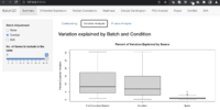
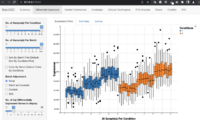
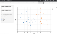
BatchQC tool

• https://www.bioconductor.org/packages/release/bioc/html/BatchQC.html
• What is Explained Variance? (Definition & Example)
  • The explained variance can be found in the SS (“sum of squares”) column for the Between Groups variation.
  • In a regression model, the explained variance is summarized by R-squared, often written R2 = SSR/SST; Coefficient of Determination.
• Some screenshots

AMDBNorm - adjustment mean distribution-based normalization

AMDBNorm: an approach based on distribution adjustment to eliminate batch effects of gene expression data Zhang, Briefings in Bioinformatics 2021

AMDBNorm assumes that each sample in the biologic condition has the same distribution.

It selects a reference batch in advance, then

1. aligns other batches with the distribution of the reference batch, and finally
2. corrects the gene expression according to their mean values in the reference batch so that the expression of each gene in each batch is at the same level.

Evaluation methods

• Visualization by principal component analysis
• Evaluation of batch effects by BatchQC software
• Principal variance component analysis
• Hierarchical cluster analysis
• Sensitivity analysis of AMDBNorm to reference batch
• Adaptability analysis of batch correction methods to the new samples

TCGA

TCGAbatch_Correction()

Confounding factors

AC-PCoA: Adjustment for confounding factors using principal coordinate analysis 2022

impute.knn

• ?impute.knn impute.knn(data ,k = 10, rowmax = 0.5, colmax = 0.8, maxp = 1500, rng.seed=362436069)
  • rowmax: The maximum percent missing data allowed in any row (default 50%). For any rows with more than rowmax% missing are imputed using the overall mean per sample.
  • colmax: The maximum percent missing data allowed in any column (default 80%). If any column has more than colmax% missing data, the program halts and reports an error.
  Why are missing values on row 3 imputed by 0?

  BiocManager::install("impute")
  library(impute)
  
  set.seed(1)
  x <- matrix(rnorm(10*4), nr=10)
  x[1,1] <- NA
  x[2,1:2] <- NA
  x[3,1:3] <- NA
  x[1:9, 1] <- NA
  x2 <- impute.knn(x, k=2)
  # Error in impute.knn(x, k = 2) : 
  #   a column has more than 80 % missing values!
  
  set.seed(1)
  x <- matrix(rnorm(10*4), nr=10)
  x[1,1] <- NA
  x[2,1:2] <- NA
  x[3,1:3] <- NA
  x2 <- impute.knn(x, k=2)
  # Warning message:
  #   In knnimp(x, k, maxmiss = rowmax, maxp = maxp) :
  #   1 rows with more than 50 % entries missing;
  # mean imputation used for these rows
  names(x2)
  [1] "data"      "rng.seed"  "rng.state"
  head(x2$data)
  #            [,1]        [,2]        [,3]        [,4]
  # [1,]  0.1351965  1.51178117  0.91897737  1.35867955
  # [2,] -0.5629284  0.27448386  0.78213630 -0.10278773
  # [3,]  0.0000000  0.00000000  0.00000000  0.38767161
  # [4,]  1.5952808 -2.21469989 -1.98935170 -0.05380504
  # [5,]  0.3295078  1.12493092  0.61982575 -1.37705956
  
  set.seed(1)
  x <- 2^matrix(rnorm(10*4), nr=10)
  x[1,1] <- NA
  x[2,1:2] <- NA
  x[3,1:3] <- NA
  x2 <- impute.knn(x, k=2)
  head(x2$data)
  
  x3 <- impute.knn(x, k=2)
  identical(x2$data, x3$data) # true

  Another case that we are able to verify imputed for rows with more than rowmax% missing values. Two rows satisfy the condition. Note the missing value on row 3, column 3 is computed by excluding ALL rows satisfying the condition.

  set.seed(1)
  x <- matrix(rnorm(10*4), nr=10)
  x[1,1] <- NA
  x[2,1:2] <- NA
  x[3,1:3] <- NA
  
  x2 <- impute.knn(x, k=2, rowmax=.25)
  head(x2$data)
  #            [,1]        [,2]        [,3]        [,4]
  # [1,]  0.1351965  1.51178117  0.91897737  1.35867955
  # [2,]  0.3714953  0.33998088  0.78213630 -0.10278773
  # [3,]  0.3714953  0.33998088 -0.27417921  0.38767161
  # [4,]  1.5952808 -2.21469989 -1.98935170 -0.05380504
  
  mean(x[,1], na.rm = T)
  # [1] 0.3714953  # same
  mean(x[,2], na.rm = T)
  # [1] 0.3399809  # same 
  mean(x[,3], na.rm = T)
  # [1] -0.1568108 # not the same
  
  mean(x[-c(2,3),3], na.rm = T)
  # [1] -0.2741792 # same