Glmnet
Basic
- https://en.wikipedia.org/wiki/Lasso_(statistics). It has a discussion when two covariates are highly correlated. For example if gene [math]\displaystyle{ i }[/math] and gene [math]\displaystyle{ j }[/math] are identical, then the values of [math]\displaystyle{ \beta _{j} }[/math] and [math]\displaystyle{ \beta _{k} }[/math] that minimize the lasso objective function are not uniquely determined. Elastic Net has been designed to address this shortcoming.
- Strongly correlated covariates have similar regression coefficients, is referred to as the grouping effect. From the wikipedia page "one would like to find all the associated covariates, rather than selecting only one from each set of strongly correlated covariates, as lasso often does. In addition, selecting only a single covariate from each group will typically result in increased prediction error, since the model is less robust (which is why ridge regression often outperforms lasso)".
- Glmnet Vignette. It tries to minimize [math]\displaystyle{ RSS(\beta) + \lambda [(1-\alpha)\|\beta\|_2^2/2 + \alpha \|\beta\|_1] }[/math]. The elastic-net penalty is controlled by [math]\displaystyle{ \alpha }[/math], and bridge the gap between lasso ([math]\displaystyle{ \alpha = 1 }[/math]) and ridge ([math]\displaystyle{ \alpha = 0 }[/math]). Following is a CV curve (adaptive lasso) using the example from glmnet(). Two vertical lines are indicated: left one is lambda.min (that gives minimum mean cross-validated error) and right one is lambda.1se (the most regularized model such that error is within one standard error of the minimum). For the tuning parameter [math]\displaystyle{ \lambda }[/math],
- The larger the [math]\displaystyle{ \lambda }[/math], more coefficients are becoming zeros (think about coefficient path plots) and thus the simpler (more regularized) the model.
- If [math]\displaystyle{ \lambda }[/math] becomes zero, it reduces to the regular regression and if [math]\displaystyle{ \lambda }[/math] becomes infinity, the coefficients become zeros.
- In terms of the bias-variance tradeoff, the larger the [math]\displaystyle{ \lambda }[/math], the higher the bias and the lower the variance of the coefficient estimators.
File:Glmnetplot.svg File:Glmnet path.svg File:Glmnet l1norm.svg
set.seed(1010)
n=1000;p=100
nzc=trunc(p/10)
x=matrix(rnorm(n*p),n,p)
beta=rnorm(nzc)
fx= x[,seq(nzc)] %*% beta
eps=rnorm(n)*5
y=drop(fx+eps)
px=exp(fx)
px=px/(1+px)
ly=rbinom(n=length(px),prob=px,size=1)

## Full lasso
set.seed(999)
cv.full <- cv.glmnet(x, ly, family='binomial', alpha=1, parallel=TRUE)
plot(cv.full)  # cross-validation curve and two lambda's
plot(glmnet(x, ly, family='binomial', alpha=1), xvar="lambda", label=TRUE) # coefficient path plot
plot(glmnet(x, ly, family='binomial', alpha=1))  # L1 norm plot
log(cv.full$lambda.min) # -4.546394
log(cv.full$lambda.1se) # -3.61605
sum(coef(cv.full, s=cv.full$lambda.min) != 0) # 44

## Ridge Regression to create the Adaptive Weights Vector
set.seed(999)
cv.ridge <- cv.glmnet(x, ly, family='binomial', alpha=0, parallel=TRUE)
wt <- 1/abs(matrix(coef(cv.ridge, s=cv.ridge$lambda.min)
                   [, 1][2:(ncol(x)+1)] ))^1 ## Using gamma = 1, exclude intercept
## Adaptive Lasso using the 'penalty.factor' argument
set.seed(999)
cv.lasso <- cv.glmnet(x, ly, family='binomial', alpha=1, parallel=TRUE, penalty.factor=wt)
# defautl type.measure="deviance" for logistic regression
plot(cv.lasso)
log(cv.lasso$lambda.min) # -2.995375
log(cv.lasso$lambda.1se) # -0.7625655
sum(coef(cv.lasso, s=cv.lasso$lambda.min) != 0) # 34
- cv.glmnet() has a logical parameter parallel which is useful if a cluster or cores have been previously allocated
- Ridge regression and the LASSO
- Standard error/Confidence interval
- Standard Errors in GLMNET and Confidence intervals for Ridge regression
- Why SEs are not meaningful and are usually not provided in penalized regression?
- Hint: standard errors are not very meaningful for strongly biased estimates such as arise from penalized estimation methods.
- Penalized estimation is a procedure that reduces the variance of estimators by introducing substantial bias.
- The bias of each estimator is therefore a major component of its mean squared error, whereas its variance may contribute only a small part.
- Any bootstrap-based calculations can only give an assessment of the variance of the estimates.
- Reliable estimates of the bias are only available if reliable unbiased estimates are available, which is typically not the case in situations in which penalized estimates are used.
- Hottest glmnet questions from stackexchange.
- Standard errors for lasso prediction. There might not be a consensus on a statistically valid method of calculating standard errors for the lasso predictions.
- Code for Adaptive-Lasso for Cox's proportional hazards model by Zhang & Lu (2007). This can compute the SE of estimates. The weights are originally based on the maximizers of the log partial likelihood. However, the beta may not be estimable in cases such as high-dimensional gene data, or the beta may be unstable if strong collinearity exists among covariates. In such cases, robust estimators such as ridge regression estimators would be used to determine the weights.
- Some issues:
- With group of highly correlated features, Lasso tends to select amongst them arbitrarily.
- Often empirically ridge has better predictive performance than lasso but lasso leads to sparser solution
- Elastic-net (Zou & Hastie '05) aims to address these issues: hybrid between Lasso and ridge regression, uses L1 and L2 penalties.
- Gradient-Free Optimization for GLMNET Parameters
- Gsslasso Cox: a Bayesian hierarchical model for predicting survival and detecting associated genes by incorporating pathway information, Tang et al BMC Bioinformatics 2019
- Outlier detection and robust variable selection via the penalized weighted LAD-LASSO method Jiang 2020
- LASSO REGRESSION (HOME MADE)
- Course notes on Optimization for Machine Learning
- How to calculate R Squared value for Lasso regression using glmnet in R
Lambda [math]\displaystyle{ \lambda }[/math]
- A list of potential lambdas: see Linear Regression case. The λ sequence is determined by lambda.max and lambda.min.ratio.
- lambda.max is computed from the input x and y; it is the smallest value for lambda such that all the coefficients are zero.
- lambda.min.ratio (default is ifelse(nobs<nvars,0.01,0.0001)) is the ratio of smallest value of the generated λ sequence (say lambda.min) to lambda.max.
- The program then generated nlambda values linear on the log scale from lambda.max down to lambda.min.
- Choosing hyper-parameters (α and λ) in penalized regression by Florian Privé
- lambda.min vs lambda.1se
- The lambda.1se represents the value of λ in the search that was simpler than the best model (lambda.min), but which has error within 1 standard error of the best model ( lambda.min < lambda.1se ). In other words, using the value of lambda.1se as the selected value for λ results in a model that is slightly simpler than the best model but which cannot be distinguished from the best model in terms of error given the uncertainty in the k-fold CV estimate of the error of the best model.
- lambda.1se not being in one standard error of the error When we say 1 standard error, we are not talking about the standard error across the lambda's but the standard error across the folds for a given lambda.
- The lambda.min option refers to value of λ at the lowest CV error. The error at this value of λ is the average of the errors over the k folds and hence this estimate of the error is uncertain.
- https://www.rdocumentation.org/packages/glmnet/versions/2.0-10/topics/glmnet
- glmnetUtils: quality of life enhancements for elastic net regression with glmnet
- Mixing parameter: alpha=1 is the lasso penalty, and alpha=0 the ridge penalty and anything between 0–1 is Elastic net.
- RIdge regression uses Euclidean distance/L2-norm as the penalty. It won't remove any variables.
- Lasso uses L1-norm as the penalty. Some of the coefficients may be shrunk exactly to zero.
- In ridge regression and lasso, what is lambda?
- Lambda is a penalty coefficient. Large lambda will shrink the coefficients.
- cv.glment()$lambda.1se gives the most regularized model such that error is within one standard error of the minimum
- A deep dive into glmnet: penalty.factor, standardize, offset
- Lambda sequence is not affected by the "penalty.factor"
- How "penalty.factor" used by the objective function may need to be corrected
- A deep dive into glmnet: predict.glmnet
Mixing parameter [math]\displaystyle{ \alpha }[/math]
cva.glmnet() from the glmnetUtils package to choose both the alpha and lambda parameters via cross-validation, following the approach described in the help page for cv.glmnet.
Underfittig, overfitting and relaxed lasso
- https://cran.r-project.org/web/packages/glmnet/vignettes/relax.pdf
- The Relaxed Lasso: A Better Way to Fit Linear and Logistic Models
- Overfitting: small lambda, lots of non-zero coefficients
- Underfitting: large lambda, not enough variables
- Relaxed Lasso by Nicolai Meinshausen
- Why is “relaxed lasso” different from standard lasso?
- https://web.stanford.edu/~hastie/TALKS/hastieJSM2017.pdf#page=13
- Stabilizing the lasso against cross-validation variability
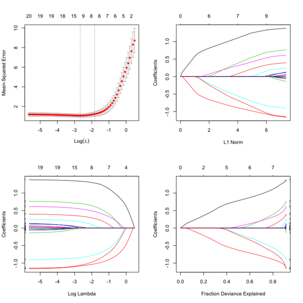
Plots
library(glmnet)
data(QuickStartExample)

cvfit = cv.glmnet(x, y)
fit = glmnet(x, y)

oldpar <- par(mfrow=c(2,2))
plot(cvfit) # mse vs log(lambda)
plot(fit) # coef vs L1 norm
plot(fit, xvar = "lambda", label = TRUE) # coef vs log(lambda)
plot(fit, xvar = "dev", label = TRUE) # coef vs Fraction Deviance Explained
par(oldpar)
print() method
?print.glmnet and ?print.cv.glmnet
Extract/compute deviance
deviance(fitted_glmnet_object)

coxnet.deviance(pred = NULL, y, x = 0, offset = NULL,
  weights = NULL, beta = NULL)
cv.glmnet
Usage
cv.glmnet(x, y, weights = NULL, offset = NULL, lambda = NULL,
  type.measure = c("default", "mse", "deviance", "class", "auc", "mae",
  "C"), nfolds = 10, foldid = NULL, alignment = c("lambda",
  "fraction"), grouped = TRUE, keep = FALSE, parallel = FALSE,
  gamma = c(0, 0.25, 0.5, 0.75, 1), relax = FALSE, trace.it = 0, ...)
type.measure parameter (loss to use for CV):
- default = deviance which uses squared-error for gaussian models (a.k.a type.measure="mse"), logistic and poisson regresion, and partial-likelihood for the Cox model. PS: for binary response data I found that type='class' gives a discontinuous CV curve while 'deviance' give a smooth CV curve.
- mse or mae (mean absolute error) can be used by all models except the "cox"; they measure the deviation from the fitted mean to the response
- class applies to binomial and multinomial logistic regression only, and gives misclassification error.
- auc is for two-class logistic regression only, and gives area under the ROC curve.
- C is Harrel's concordance measure, only available for cox models
No need for glmnet if we have run cv.glmnet
https://stats.stackexchange.com/a/77549 Do not supply a single value for lambda. Supply instead a decreasing sequence of lambda values. glmnet relies on its warms starts for speed, and its often faster to fit a whole path than compute a single fit.
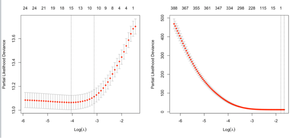
cv.glmnet in cox model
Note that the y-axis on the plot depends on the type.measure parameter. It is not the objective function used to find the estimator.
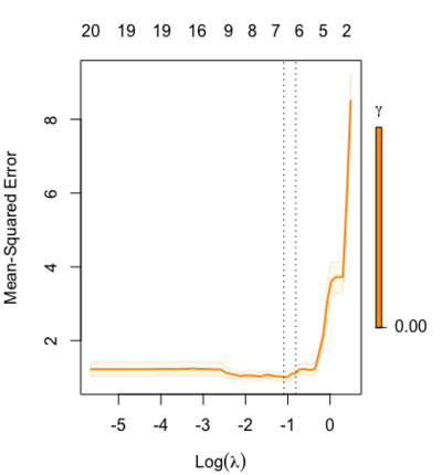
It is not always partial likelihood device has a largest value at a large lambda. In the following two plots, the first one is from the glmnet vignette and the 2nd one is from the coxnet vignette.
Relaxed fit and [math]\displaystyle{ \gamma }[/math] parameter
https://cran.r-project.org/web/packages/glmnet/vignettes/relax.pdf
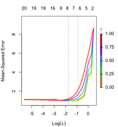
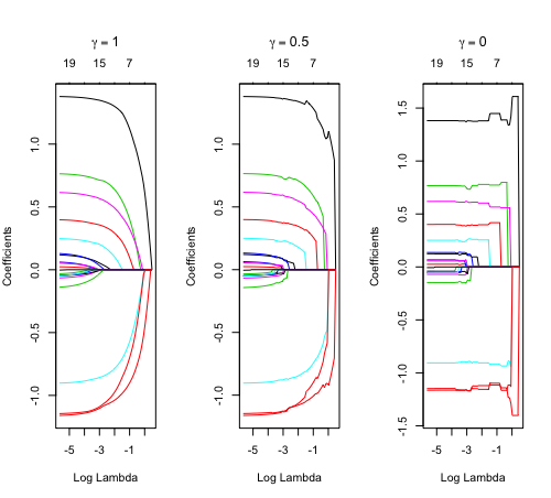
Relaxed fit: Take a glmnet fitted object, and then for each lambda, refit the variables in the active set without any penalization.
Suppose the glmnet fitted linear predictor at [math]\displaystyle{ \lambda }[/math] is [math]\displaystyle{ \hat\eta_\lambda(x) }[/math] and the relaxed version is [math]\displaystyle{ \tilde\eta_\lambda(x) }[/math]. We also allow for shrinkage between the two:
- [math]\displaystyle{ \begin{align} \tilde \eta_{\lambda,\gamma}= \gamma\hat\eta_\lambda(x) + (1-\gamma)\tilde\eta_\lambda(x). \end{align} }[/math]
[math]\displaystyle{ \gamma\in[0,1] }[/math] is an additional tuning parameter which can be selected by cross validation.
The debiasing will potentially improve prediction performance, and CV will typically select a model with a smaller number of variables.
The default behavior of extractor functions like predict and coef, as well as plot will be to present results from the glmnet fit (not cv.glmnet), unless a value of [math]\displaystyle{ \gamma }[/math] is given different from the default value [math]\displaystyle{ \gamma=1 }[/math].
Question: how does cv.glmnet() select [math]\displaystyle{ \gamma }[/math] parameter? Ans: it depends on the parameter type.measure in cv.glmnet.
library(glmnet) data(QuickStartExample) fitr=glmnet(x,y, relax=TRUE) set.seed(1) cfitr=cv.glmnet(x,y,relax=TRUE) c(fitr$lambda.min, fitr$lambda.1se) # [1] 0.08307327 0.15932708 str(cfitr$relaxed) plot(cfitr),oldpar <- par(mfrow=c(1,3), mar = c(5,4,6,2)) plot(fitr, main = expression(gamma == 1)) plot(fitr,gamma=0.5, main = expression(gamma == .5)) plot(fitr,gamma=0, main = expression(gamma == 0)) par(oldpar) |
Special cases:
set.seed(1) cfitr2=cv.glmnet(x,y,gamma=0,relax=TRUE) # default gamma = c(0, 0.25, 0.5, 0.75, 1) plot(cfitr2) c(cfitr2$lambda.min, cfitr2$lambda.1se) # [1] 0.08307327 0.15932708 str(cfitr2$relaxed) |
Computation time
beta1 = 2; beta2 = -1
lambdaT = .002 # baseline hazard
lambdaC = .004  # hazard of censoring
set.seed(1234)
x1 = rnorm(n)
x2 = rnorm(n)
# true event time
T = Vectorize(rweibull)(n=1, shape=1, scale=lambdaT*exp(-beta1*x1-beta2*x2))
# No censoring
event2 <- rep(1, length(T))

system.time(fit <- cv.glmnet(x, Surv(T,event2), family = 'cox'))
#    user  system elapsed
#   4.701   0.016   4.721
system.time(fitr <- cv.glmnet(x, Surv(T,event2), family = 'cox', relax= TRUE))
#    user  system elapsed
# 161.002   0.382 161.573
predict() and coef() methods
?predict.glmnet OR ?coef.glmnet OR ?coef.relaxed. Similar to other predict methods, this functions predicts fitted values, logits, coefficients and more from a fitted "glmnet" object.
## S3 method for class 'glmnet'
predict(object, newx, s = NULL, type = c("link",
  "response", "coefficients", "nonzero", "class"), exact = FALSE,
  newoffset, ...)

## S3 method for class 'relaxed'
predict(object, newx, s = NULL, gamma = 1,
  type = c("link", "response", "coefficients", "nonzero", "class"),
  exact = FALSE, newoffset, ...)
## S3 method for class 'glmnet'
coef(object, s = NULL, exact = FALSE, ...)
?predict.cv.glmnet OR ?coef.cv.glmnet OR ?coef.cv.relaxed. This function makes predictions from a cross-validated glmnet model, using the stored "glmnet.fit" object, and the optimal value chosen for lambda (and gamma for a 'relaxed' fit).
## S3 method for class 'cv.glmnet'
predict(object, newx, s = c("lambda.1se",
  "lambda.min"), ...)

## S3 method for class 'cv.relaxed'
predict(object, newx, s = c("lambda.1se",
  "lambda.min"), gamma = c("gamma.1se", "gamma.min"), ...)
Cindex
https://www.rdocumentation.org/packages/glmnet/versions/3.0-2/topics/Cindex
Usage:
Cindex(pred, y, weights = rep(1, nrow(y)))
assess.glmnet
https://www.rdocumentation.org/packages/glmnet/versions/3.0-2/topics/assess.glmnet
Usage:
assess.glmnet(object, newx = NULL, newy, weights = NULL,
  family = c("gaussian", "binomial", "poisson", "multinomial", "cox",
  "mgaussian"), ...)
confusion.glmnet(object, newx = NULL, newy, family = c("binomial",
  "multinomial"), ...)

roc.glmnet(object, newx = NULL, newy, ...)
ridge regression
# example from SGL package
set.seed(1)
n = 50; p = 100; size.groups = 10
X = matrix(rnorm(n * p), ncol = p, nrow = n)
beta = (-2:2)
y = X[,1:5] %*% beta + 0.1*rnorm(n)
data = list(x = X, y = y)

cvfit <- cv.glmnet(X, y, alpha = 0)
plot(cvfit)

o <- coef(cvfit, lambda = cvfit$lambda.min) %>% drop()

sum(o != 0) # [1] 101.
            # Too biased.
o[1:10]
#   (Intercept)            V1            V2            V3            V4
# -3.269401e-01 -2.253226e-36 -8.900799e-37  5.198885e-37  1.311976e-36
#            V5            V6            V7            V8            V9
#  1.873125e-36  1.582532e-37  2.085781e-37  4.732839e-37  2.997614e-37

y_predicted <- predict(cvfit, s = cvfit$lambda.min, newx = X)
# Sum of Squares Total and Error
sst <- sum((y - mean(y))^2)
sse <- sum((y_predicted - y)^2)
# R squared
rsq <- 1 - sse / sst
rsq  # 0.46

library(SGL)  # sparse group lasso
set.seed(1)
index <- ceiling(1:p / size.groups)
cvFit = cvSGL(data, index, type = "linear", alpha=.95) # this alpha is the default
plot(cvFit)
cvFit$fit$beta[, 20] # 20th lambda gives smallest negative log likelihood
                     # identify correct predictors
#  [1] -10.942712  -6.167799   0.000000   6.595406  14.442019   0.000000 ...

set.seed(1)
cvFit2 = cvSGL(data, index, type = "linear", alpha=0)
plot(cvFit2)
cvFit2$fit$beta[, 20]
#  [1] -10.8417371  -6.5251240   0.2476438   6.7223001  14.1605263   0.2149542
#  [7]   0.2481450   0.1404282   0.1799818   0.3784596   0.0000000   0.0000000 ...
- Tikhonov regularization (ridge regression). It was used to handle ill-posed/overfitting situation. Ridge regression shrinks the coefficients by a uniform factor of [math]\displaystyle{ {\displaystyle (1+N\lambda )^{-1}}{\displaystyle (1+N\lambda )^{-1}} }[/math] and does not set any coefficients to zero.
- cvSGL
- How and when: ridge regression with glmnet. On training data, ridge regression fits less well than the OLS but the parameter estimate is more stable. So it does better in prediction because it is less sensitive to extreme variance in the data such as outliers.
Group lasso
- grplasso package. Why use group lasso instead of lasso? Already for the special case in linear regression when not only continuous but also categorical predictors (factors) are present, the lasso solution is not satisfactory as it only selects individual dummy variables instead of whole factors. Moreover, the lasso solution depends on how the dummy variables are encoded. Choosing different contrasts for a categorical predictor will produce different solutions in general.
- SGL
- MSGLasso
Adaptive lasso and weights
Oracle property and adaptive lasso
- Variable Selection via Nonconcave Penalized Likelihood and Its Oracle Properties, Fan & Li (2001) JASA
- Adaptive Lasso: What it is and how to implement in R. Adaptive lasso weeks to minimize [math]\displaystyle{ RSS(\beta) + \lambda \sum_1^p \hat{\omega}_j |\beta_j| }[/math] where [math]\displaystyle{ \lambda }[/math] is the tuning parameter, [math]\displaystyle{ \hat{\omega}_j = \frac{1}{(|\hat{\beta}_j^{ini}|)^\gamma} }[/math] is the adaptive weights vector and [math]\displaystyle{ \hat{\beta}_j^{ini} }[/math] is an initial estimate of the coefficients obtained through ridge regression. Adaptive Lasso ends up penalizing more those coefficients with lower initial estimates. [math]\displaystyle{ \gamma }[/math] is a positive constant for adjustment of the adaptive weight vector, and the authors suggest the possible values of 0.5, 1 and 2.
- When n goes to infinity, [math]\displaystyle{ \hat{\omega}_j |\beta_j| }[/math] converges to [math]\displaystyle{ I(\beta_j \neq 0) }[/math]. So the adaptive Lasso procedure can be regarded as an automatic implementation of best-subset selection in some asymptotic sense.
- What is the oracle property of an estimator? An oracle estimator must be consistent in 1) variable selection and 2) consistent parameter estimation.
- (Linear regression) The adaptive lasso and its oracle properties Zou (2006, JASA)
- (Cox model) Adaptive-LASSO for Cox's proportional hazard model by Zhang and Lu (2007, Biometrika)
- When the LASSO fails???. Adaptive lasso is used to demonstrate its usefulness.
Cyclic coordinate descent
A deep dive into glmnet: type.gaussian
Survival data
- The sum of errors term can be replaced with [math]\displaystyle{ -l(\beta, \gamma) }[/math], where [math]\displaystyle{ l(\cdot, \cdot) }[/math] stands for the log-likelihood function and [math]\displaystyle{ \gamma }[/math] for the intercept. See The lasso method for variable selection in the cox model 1997.
- Regularization Paths for Cox's Proportional Hazards Model via Coordinate Descent Noah Simon, Jerome H. Friedman, Trevor Hastie, Rob Tibshirani, 2011
- Cox regression: Estimation by Patrick Breheny
- Another implementation coxnet
- Gradient lasso for Cox proportional hazards model
- Prediction method. ?predict.cv.glmnet is not clear. ?coef.glmnet is more clear.
data(CoxExample)
dim(x) # 1000 x 30
ind.train <- 1:nrow(x)/2
cv.fit <- cv.glmnet(x[ind.train, ], y[ind.train, ], family="cox")
coef(cv.fit, s = "lambda.min")
    # 30 x 1, coef(...) is equivalent to predict(type="coefficients",...)
pr <- predict(cv.fit, x[-ind.train, ], type = "link", s = "lambda.min")
    # the default option for type is 'link' which gives the linear predictors for "cox" models.
pr2 <- x[-ind.train, ] %*% coef(cv.fit, s = "lambda.min")
all.equal(pr[, 1], pr2[, 1]) # [1] TRUE
class(pr) # [1] "matrix"
class(pr2) # [1] "dgeMatrix"
# we can also use predict() with glmnet object
pr22 <- predict(fit, x[-ind.train, ], type='link', s = cv.fit$lambda.min)
all.equal(pr[, 1], pr22[, 1]) # [1] TRUE

pr3 <- predict(cv.fit, x[-ind.train, ], type = "response", s = "lambda.min")
range(pr3)  # relative risk [1]  0.05310623 19.80143519
Timing
nvec <- c(100, 400)
pvec <- c(1000, 5000)
for(n in nvec)
  for(p in pvec) {
    nzc = trunc(p/10)  # 1/10 variables are non-zeros
    x = matrix(rnorm(n * p), n, p)
    beta = rnorm(nzc)
    fx = x[, seq(nzc)] %*% beta/3
    hx = exp(fx)
    ty = rexp(n, hx)
    tcens = rbinom(n = n, prob = 0.3, size = 1)  # censoring indicator
    y = cbind(time = ty, status = 1 - tcens)  # y=Surv(ty,1-tcens) with library(survival)
    foldid = sample(rep(seq(10), length = n))
    o <- system.time(fit1_cv <- cv.glmnet(x, y, family = "cox", foldid = foldid) )
    cat(sprintf("n=%1d, p=%5d, time=%8.3f\n", n, p, o['elapsed']))
}
Running on core i7 2.6GHz, macbook pro 2018. Unit is seconds.
| p ∖ n | 100 | 400 |
|---|---|---|
| 1000 | 5 | 58 |
| 5000 | 9 | 96 |
Xeon E5-2680 v4 @ 2.40GHz
| p ∖ n | 100 | 400 |
|---|---|---|
| 1000 | 7 | 98 |
| 5000 | 13 | 125 |
Discussion
- https://stackoverflow.com/questions/tagged/glmnet
- https://stats.stackexchange.com/questions/tagged/glmnet
Prediction
- Comparison of pathway and gene-level models for cancer prognosis prediction Zheng, 2020
- CAncer bioMarker Prediction Pipeline (CAMPP)—A standardized framework for the analysis of quantitative biological data Terkelsen, 2020
LASSO vs Least angle regression
- https://web.stanford.edu/~hastie/Papers/LARS/LeastAngle_2002.pdf
- Least Angle Regression, Forward Stagewise and the Lasso
- https://www.quora.com/What-is-Least-Angle-Regression-and-when-should-it-be-used
- A simple explanation of the Lasso and Least Angle Regression
- https://stats.stackexchange.com/questions/4663/least-angle-regression-vs-lasso
- https://cran.r-project.org/web/packages/lars/index.html
Tidymodel
Lasso regression using tidymodels and #tidytuesday data for the office
Binary particle swarm optimization (BPSO)
An efficient gene selection method for microarray data based on LASSO and BPSO
