Glmnet: Difference between revisions
(→Basic) |
|||
| (82 intermediate revisions by the same user not shown) | |||
| Line 23: | Line 23: | ||
## Full lasso | ## Full lasso | ||
library(doParallel) | |||
registerDoParallel(cores = 2) | |||
set.seed(999) | set.seed(999) | ||
cv.full <- cv.glmnet(x, ly, family='binomial', alpha=1, parallel=TRUE) | cv.full <- cv.glmnet(x, ly, family='binomial', alpha=1, parallel=TRUE) | ||
| Line 39: | Line 41: | ||
## Adaptive Lasso using the 'penalty.factor' argument | ## Adaptive Lasso using the 'penalty.factor' argument | ||
set.seed(999) | set.seed(999) | ||
cv.lasso <- cv.glmnet(x, ly, family='binomial', alpha=1, parallel=TRUE, penalty.factor=wt) | cv.lasso <- cv.glmnet(x, ly, family='binomial', alpha=1, parallel=TRUE, | ||
penalty.factor=wt) | |||
# defautl type.measure="deviance" for logistic regression | # defautl type.measure="deviance" for logistic regression | ||
plot(cv.lasso) | plot(cv.lasso) | ||
| Line 71: | Line 74: | ||
* [https://myweb.uiowa.edu/pbreheny/7600/s16/notes.html High dimensional data analysis] course by P. Breheny | * [https://myweb.uiowa.edu/pbreheny/7600/s16/notes.html High dimensional data analysis] course by P. Breheny | ||
* [https://stackoverflow.com/questions/50610895/how-to-calculate-r-squared-value-for-lasso-regression-using-glmnet-in-r How to calculate R Squared value for Lasso regression using glmnet in R] | * [https://stackoverflow.com/questions/50610895/how-to-calculate-r-squared-value-for-lasso-regression-using-glmnet-in-r How to calculate R Squared value for Lasso regression using glmnet in R] | ||
* [https://stackoverflow.com/a/43746925 Getting AIC/BIC/Likelihood from GLMNet] | * [https://stackoverflow.com/a/43746925 Getting AIC/BIC/Likelihood from GLMNet], [https://stackoverflow.com/q/69104789 AIC comparison in glmnet]. | ||
* Specifying categorical predictors in glmnet() - [https://stats.stackexchange.com/a/72271 an example]. The new solution is to use the '''makeX()''' function; see the vignette. | |||
== Lambda <math>\lambda</math> == | == Lambda <math>\lambda</math> == | ||
| Line 77: | Line 81: | ||
<li>A list of potential lambdas: see [http://web.stanford.edu/~hastie/glmnet/glmnet_alpha.html#lin Linear Regression] case. The λ sequence is determined by '''lambda.max''' and '''lambda.min.ratio'''. | <li>A list of potential lambdas: see [http://web.stanford.edu/~hastie/glmnet/glmnet_alpha.html#lin Linear Regression] case. The λ sequence is determined by '''lambda.max''' and '''lambda.min.ratio'''. | ||
<ul> | <ul> | ||
<li>'''lambda.max''' is computed from the input x and y; it is the maximal value for ''lambda'' such that all the coefficients are zero. [https://stackoverflow.com/a/26617280 How does glmnet compute the maximal lambda value?]. However see the [[#Random_data|Random data example]]. </li> | <li>'''lambda.max''' is computed from the input x and y; it is the maximal value for ''lambda'' such that all the coefficients are zero. [https://stackoverflow.com/a/26617280 How does glmnet compute the maximal lambda value?] & [https://stats.stackexchange.com/a/174907 Choosing the range and grid density for regularization parameter in LASSO]. However see the [[#Random_data|Random data example]]. </li> | ||
<li>'''lambda.min.ratio''' (default is ifelse(nobs<nvars,0.01,0.0001)) is the ratio of smallest value of the generated λ sequence (say ''lambda.min'') to ''lambda.max''. </li> | <li>'''lambda.min.ratio''' (default is ifelse(nobs<nvars,0.01,0.0001)) is the ratio of smallest value of the generated λ sequence (say ''lambda.min'') to ''lambda.max''. </li> | ||
<li>The program then generated ''nlambda'' values linear on the log scale from ''lambda.max'' down to ''lambda.min''. </li> | <li>The program then generated ''nlambda'' values linear on the log scale from ''lambda.max'' down to ''lambda.min''. </li> | ||
| Line 136: | Line 140: | ||
=== Multiple seeds in cross-validation === | === Multiple seeds in cross-validation === | ||
<ul> | |||
<li>[https://stats.stackexchange.com/a/103144 Variablity in cv.glmnet results]. From the cv.glmnet() reference manual: ''Note also that the results of cv.glmnet are random, since the folds are selected at random. Users can reduce this randomness by running cv.glmnet many times, and '''averaging the error curves'''. '' | |||
<pre> | |||
MSEs <- NULL | |||
for (i in 1:100){ | |||
cv <- cv.glmnet(y, x, alpha=alpha, nfolds=k) | |||
MSEs <- cbind(MSEs, cv$cvm) | |||
} | |||
rownames(MSEs) <- cv$lambda | |||
lambda.min <- as.numeric(names(which.min(rowMeans(MSEs)))) | |||
</pre> | |||
<li>[https://www.sciencedirect.com/science/article/pii/S016794731300323X Stabilizing the lasso against cross-validation variability] | |||
<li>[https://github.com/cran/caret/blob/master/R/trainControl.R caret::trainControl(.., repeats, ...)] | |||
</pre> | |||
=== Cross Validated LASSO: What are its weaknesses? === | |||
[https://www.reddit.com/r/rstats/comments/bz7qdq/cross_validated_lasso_with_the_glmnet_package/ Cross Validated LASSO with the glmnet package: What are its weaknesses?] | |||
=== At what lambda is each coefficient shrunk to 0 === | |||
[https://stackoverflow.com/a/73312496 glmnet: at what lambda is each coefficient shrunk to 0?] | |||
== Mixing parameter <math>\alpha</math> == | == Mixing parameter <math>\alpha</math> == | ||
| Line 185: | Line 206: | ||
See also [[Survival_data#glmnet|Survival → glmnet]]. | See also [[Survival_data#glmnet|Survival → glmnet]]. | ||
=== coefplot: Plots Coefficients from Fitted Models === | |||
* https://cran.r-project.org/web/packages/coefplot/index.html | |||
* [https://www.jaredlander.com/2018/02/using-coefplot-with-glmnet/ Using coefplot with glmnet] | |||
== cv.glmnet and deviance == | == cv.glmnet and deviance == | ||
| Line 198: | Line 223: | ||
'''type.measure''' parameter (loss to use for CV): | '''type.measure''' parameter (loss to use for CV): | ||
* '''default''' | * '''default''' | ||
** type.measure = '''deviance''' which uses squared-error for gaussian models (a.k.a type.measure="mse"), logistic and poisson regression (''PS'': for binary response data I found that type='class' gives a discontinuous CV curve while 'deviance' give a smooth CV curve), | ** type.measure = '''deviance''' which uses squared-error for gaussian models (a.k.a type.measure="mse"), logistic and poisson regression (''PS'': for binary response data I found that type='class' gives a discontinuous CV curve while 'deviance' give a smooth CV curve), [https://stats.stackexchange.com/a/138524 deviance formula] for binomial model which is the same as the formula shown [https://www.ncbi.nlm.nih.gov/pmc/articles/PMC4253302/ here] and [https://r.qcbs.ca/workshop06/book-en/binomial-glm.html binomial glm] case. | ||
** type.measure = '''partial-likelihood''' for the Cox model (<span style="color: red">note that the y-axis from plot.cv.glmnet() gives deviance but the values are quite different from what deviace() gives from a non-CV modelling</span>). | ** type.measure = '''partial-likelihood''' for the Cox model (<span style="color: red">note that the y-axis from plot.cv.glmnet() gives deviance but the values are quite different from what deviace() gives from a non-CV modelling</span>). | ||
* '''mse''' or '''mae''' (mean absolute error) can be used by all models except the "cox"; they measure the deviation from the fitted mean to the response | * '''mse''' or '''mae''' (mean absolute error) can be used by all models except the "cox"; they measure the deviation from the fitted mean to the response | ||
| Line 287: | Line 312: | ||
# [1] "C-index" | # [1] "C-index" | ||
</pre> | </pre> | ||
=== What deviance is glmnet using === | |||
[https://stats.stackexchange.com/a/135062 What deviance is glmnet using to compare values of 𝜆?] | |||
=== No need for glmnet if we have run cv.glmnet === | === No need for glmnet if we have run cv.glmnet === | ||
| Line 298: | Line 326: | ||
'''Note: the CV result may changes unless we fix the random seed.''' | '''Note: the CV result may changes unless we fix the random seed.''' | ||
Note that the y-axis on the plot depends on the ''type.measure'' parameter. It is not the objective function used to find the estimator. For survival data, the y-axis is deviance (-2*loglikelihood) [so the optimal lambda should give a minimal deviance value]. | Note that the y-axis on the plot depends on the ''type.measure'' parameter. It is not the objective function used to find the estimator. For survival data, the y-axis is (residual) '''deviance''' ('''-2*loglikelihood''', or '''RSS''' in [https://funglee.github.io/ml/slides/Lecture2-LinearReg-Notes.pdf linear regression case]) [so the optimal lambda should give a minimal deviance value]. | ||
It is not always partial likelihood device has a largest value at a large lambda. In the following two plots, the first one is from the [https://cran.r-project.org/web/packages/glmnet/vignettes/glmnet.pdf#page=32 glmnet] vignette and the 2nd one is from the [https://cran.r-project.org/web/packages/glmnet/vignettes/Coxnet.pdf#page=3 coxnet] vignette. The survival data are not sparse in both examples. | It is not always partial likelihood device has a largest value at a large lambda. In the following two plots, the first one is from the [https://cran.r-project.org/web/packages/glmnet/vignettes/glmnet.pdf#page=32 glmnet] vignette and the 2nd one is from the [https://cran.r-project.org/web/packages/glmnet/vignettes/Coxnet.pdf#page=3 coxnet] vignette. The survival data are not sparse in both examples. | ||
| Line 414: | Line 442: | ||
</pre></li> | </pre></li> | ||
</ul> | </ul> | ||
== cv.glmnet and glmnet give different coefficients == | |||
[https://stackoverflow.com/a/48516541 glmnet: same lambda but different coefficients for glmnet() & cv.glmnet()] | |||
== Number of nonzero in cv.glmnet plot is not monotonic in lambda == | |||
It is possible since this is based on CV? But if we use coef() to compute the nonzero coefficients for each lambda from the fitted model, it should be monotonic. Below is one case and the Cox regression example above is another case. | |||
[[File:Cvglmnetplot.png|300px]] | |||
== Relaxed fit and <math>\gamma</math> parameter == | == Relaxed fit and <math>\gamma</math> parameter == | ||
| Line 518: | Line 554: | ||
=== AUC === | === AUC === | ||
[https://stackoverflow.com/a/52415461 Validating AUC values in R's GLMNET package]. | <ul> | ||
<li>[https://stackoverflow.com/a/52415461 Validating AUC values in R's GLMNET package]. | |||
<pre> | <pre> | ||
fit = cv.glmnet(x = data, y = label, family = 'binomial', alpha=1, type.measure = "auc") | fit = cv.glmnet(x = data, y = label, family = 'binomial', alpha=1, type.measure = "auc") | ||
| Line 524: | Line 561: | ||
auc(label,pred) | auc(label,pred) | ||
</pre> | </pre> | ||
<li>[https://www.reddit.com/r/rprogramming/comments/sfyr6w/computing_the_auc_for_test_data_using_cvglmnet/ Computing the auc for test data using cv.glmnet] | |||
</ul> | |||
=== Cindex === | === Cindex === | ||
| Line 551: | Line 590: | ||
* [https://stackoverflow.com/questions/35461839/glmnet-variable-importance glmnet - variable importance?] Note not sure if ''caret'' considers scales of variables. | * [https://stackoverflow.com/questions/35461839/glmnet-variable-importance glmnet - variable importance?] Note not sure if ''caret'' considers scales of variables. | ||
* A plot of showing the importance of variables by ranking the variables in a heatmap [https://www.nature.com/articles/ncomms6901/figures/3 Gerstung 2015]. The plot looks nice but the way of ranking variables seems not right (not based on the optimal lambda). | * A plot of showing the importance of variables by ranking the variables in a heatmap [https://www.nature.com/articles/ncomms6901/figures/3 Gerstung 2015]. The plot looks nice but the way of ranking variables seems not right (not based on the optimal lambda). | ||
* Random forest | |||
** [https://www.randomforestsrc.org/ randomForestSRC] | |||
** [https://stats.stackexchange.com/a/496047 Random Survival Forests - How Do They Work?] | |||
** [https://avikarn.com/2020-06-26-MachineLearning_rf_glmnet/ Utilizing Machine Learning algorithms (GLMnet and Random Forest models) for Genomic Prediction of a Quantitative trait]. caret::varImp | |||
* [https://stackoverflow.com/a/64629435 glmnet variable importance | `vip` vs `varImp`] | |||
=== R-square/R2 === | === R-square/R2 and dev.ratio === | ||
<ul> | |||
<li>[https://stats.stackexchange.com/a/280965 How to calculate 𝑅2 for LASSO (glmnet)]. Use cvfit$glmnet.fit$dev.ratio. According to ?glmnet, dev.ratio is the fraction of (null) deviance explained (for "elnet", this is the R-square). | |||
<li>[https://stackoverflow.com/a/52662162 How to calculate R Squared value for Lasso regression using glmnet in R] | |||
<li>[https://en.wikipedia.org/wiki/Coefficient_of_determination Coefficient of determination] from wikipedia. R2 is the '''proportion of the variation in the dependent variable that is predictable from the independent variable(s)'''. | |||
<li>[https://stats.stackexchange.com/a/446407 What is the main difference between multiple R-squared and correlation coefficient?] It provides 4 ways (same value) to calculate R2 for multiple regression (not glmnet). | |||
<pre> | |||
fm <- lm(Y ~ X1 + X2) # regression of Y on X1 and X2 | |||
fm_null <- lm(Y ~ 1) # null model | |||
== ridge regression == | # Method 1: definition | ||
var(fitted(fm)) / var(Y) # ratio of variances | |||
# Method 2 | |||
cor(fitted(fm), Y)^2 # squared correlation | |||
# Method 3 | |||
summary(fm)$r.squared # multiple R squared | |||
# Method 4 | |||
1 - deviance(fm) / deviance(fm_null) # improvement in residual sum of squares | |||
</pre> | |||
<li> %Dev is R2 in linear regression case. [https://stackoverflow.com/a/58838761 How to calculate R Squared value for Lasso regression using glmnet in R], [https://stats.stackexchange.com/a/280965 How to calculate 𝑅2 for LASSO (glmnet)] | |||
<syntaxhighlight lang="rsplus"> | |||
library(glmnet) | |||
data(QuickStartExample) | |||
x <- QuickStartExample$x | |||
y <- QuickStartExample$y | |||
dim(x) | |||
# [1] 100 20 | |||
fit2 <- lm(y~x) | |||
summary(fit2) | |||
# Multiple R-squared: 0.9132, Adjusted R-squared: 0.8912 | |||
glmnet(x, y) | |||
# Df %Dev Lambda | |||
# 1 0 0.00 1.63100 | |||
# 2 2 5.53 1.48600 | |||
# 3 2 14.59 1.35400 | |||
# ... | |||
# 64 20 91.31 0.00464 | |||
# 65 20 91.32 0.00423 | |||
# 66 20 91.32 0.00386 | |||
# 67 20 91.32 0.00351 | |||
</syntaxhighlight> | |||
<li>An example to get R2 (deviance) from glmnet. '''%DEV''' or cv.glmnet()$glmnet.fit$dev.ratio is fraction of (null) deviance explained. [https://glmnet.stanford.edu/reference/deviance.glmnet.html ?deviance.glmnet] | |||
<pre> | |||
set.seed(1010) | |||
n=1000;p=100 | |||
nzc=trunc(p/10) | |||
x=matrix(rnorm(n*p),n,p) | |||
beta=rnorm(nzc) | |||
fx= x[,seq(nzc)] %*% beta | |||
eps=rnorm(n)*5 | |||
y=drop(fx+eps) | |||
set.seed(999) | |||
cvfit <- cv.glmnet(x, y) | |||
cvfit | |||
# Measure: Mean-Squared Error | |||
# Lambda Index Measure SE Nonzero | |||
# min 0.2096 24 24.32 0.8105 21 | |||
# 1se 0.3663 18 24.93 0.8808 12 | |||
cvfit$cvm[cvfit$lambda == cvfit$lambda.min] | |||
# 24.3218 <- mean cross-validated error | |||
cvfit$glmnet.fit | |||
# Df %Dev Lambda | |||
# 1 0 0.00 1.78100 | |||
# 2 1 1.72 1.62300 | |||
# 23 19 25.40 0.23000 | |||
# 24 21 25.96 0.20960 <- Same as glmnet() result -----------------------------+ | |||
# 25 21 26.44 0.19100 | | |||
# ... | | |||
cvfit$glmnet.fit$dev.ratio[cvfit$lambda == cvfit$lambda.min] | | |||
# [1] 0.2596395 dev.ratio=1-dev/nulldev. ?deviance.glmnet | | |||
| | |||
fit <- glmnet(x, y, lambda=cvfit$lambda.min); fit | | |||
# Df %Dev Lambda | | |||
# 1 21 25.96 0.2096 <---------------------------------------------------------+ | |||
predict.lasso <- predict(fit, newx=x, s="lambda.min", type = 'response')[,1] | | |||
| | |||
1 - deviance(fit)/deviance(lm(y~1)) | | |||
# [1] 0.2596395 <- Same as glmnet() ------------------------------------------+ | |||
deviance(lm(y~1)) # Same as sum((y-mean(y))**2) | |||
deviance(fit) # Same as sum((y-predict.lasso)**2) | |||
cor(predict.lasso, y)^2 | |||
# [1] 0.2714228 <- Not the same as glmnet() | |||
var(predict.lasso) / var(y) | |||
# [1] 0.1701002 <- Not the same as glmnet() | |||
</pre> | |||
</ul> | |||
== ridge regression and multicollinear == | |||
https://en.wikipedia.org/wiki/Ridge_regression. Ridge regression is a method of estimating the coefficients of multiple-regression models in scenarios where linearly independent variables are highly correlated. | |||
<pre> | <pre> | ||
# example from SGL package | # example from SGL package | ||
| Line 607: | Line 737: | ||
* [https://www.rdocumentation.org/packages/SGL/versions/1.3/topics/cvSGL cvSGL] | * [https://www.rdocumentation.org/packages/SGL/versions/1.3/topics/cvSGL cvSGL] | ||
* [https://drsimonj.svbtle.com/ridge-regression-with-glmnet How and when: ridge regression with glmnet]. On training data, ridge regression fits less well than the OLS but the parameter estimate is more '''stable'''. So it does better in prediction because it is less '''sensitive''' to extreme variance in the data such as outliers. | * [https://drsimonj.svbtle.com/ridge-regression-with-glmnet How and when: ridge regression with glmnet]. On training data, ridge regression fits less well than the OLS but the parameter estimate is more '''stable'''. So it does better in prediction because it is less '''sensitive''' to extreme variance in the data such as outliers. | ||
== Filtering variables == | |||
See its vignette. | |||
''One might think that unsupervised '''filtering using just x''' before fitting the model is fair game, and perhaps need not be accounted for in cross-validation. This is an interesting issue, and one can argue that there could be some bias if it was not accounted for. But '''filtering using x and y definitely introduces potential bias'''. However, it can still give good results, as long as it it correctly accounted for when running CV.'' | |||
== Graphical lasso == | |||
* [https://en.wikipedia.org/wiki/Graphical_lasso Wikipedia] | |||
* [https://scholar.google.com/scholar?hl=en&as_sdt=0%2C21&q=Sparse+inverse+covariance+estimation+with+the+graphical+lasso&btnG= Google scholar] cited by 5k. | |||
* [https://academic.oup.com/biostatistics/article/9/3/432/224260?searchresult=1 Sparse inverse covariance estimation with the graphical lasso] Friedman 2008. Number 3 of [https://academic.oup.com/biostatistics/pages/highly_cited_articles highly cited articles]. | |||
== Group lasso == | == Group lasso == | ||
| Line 613: | Line 753: | ||
* [https://cran.r-project.org/web/packages/gglasso/ gglasso]: Group Lasso Penalized Learning Using a Unified BMD Algorithm. [https://stackoverflow.com/a/51107252 Using LASSO in R with categorical variables] | * [https://cran.r-project.org/web/packages/gglasso/ gglasso]: Group Lasso Penalized Learning Using a Unified BMD Algorithm. [https://stackoverflow.com/a/51107252 Using LASSO in R with categorical variables] | ||
* [https://cran.r-project.org/web/packages/SGL/index.html SGL] | * [https://cran.r-project.org/web/packages/SGL/index.html SGL] | ||
** [https://github.com/yngvem/group-lasso Group Lasso implementation following the scikit-learn API] with nice documentation | |||
** [https://bmcbioinformatics.biomedcentral.com/articles/10.1186/s12859-020-03725-w Seagull]: lasso, group lasso and sparse-group lasso regularization for linear regression models via proximal gradient descent. [https://cran.r-project.org/web/packages/seagull/index.html CRAN]. | ** [https://bmcbioinformatics.biomedcentral.com/articles/10.1186/s12859-020-03725-w Seagull]: lasso, group lasso and sparse-group lasso regularization for linear regression models via proximal gradient descent. [https://cran.r-project.org/web/packages/seagull/index.html CRAN]. | ||
* [https://cran.r-project.org/web/packages/MSGLasso/ MSGLasso] | * [https://cran.r-project.org/web/packages/MSGLasso/ MSGLasso] | ||
* [https://cran.r-project.org/web/packages/sgPLS/ sgPLS], [https://academic.oup.com/bioinformatics/article/32/1/35/1743486#83424155 paper] Liquet 2016 | * [https://cran.r-project.org/web/packages/sgPLS/ sgPLS], [https://academic.oup.com/bioinformatics/article/32/1/35/1743486#83424155 paper] Liquet 2016 | ||
<ul> | <ul> | ||
<li> [https://cran.r-project.org/web/packages/pcLasso/ | <li> [https://cran.r-project.org/web/packages/pcLasso/ pcLasso: Principal Components Lasso] package | ||
<ul> | <ul> | ||
<li>[https://statisticaloddsandends.wordpress.com/2019/01/14/pclasso-a-new-method-for-sparse-regression/ pclasso paper], [https://kjytay.github.io/cv/pcLasso_JSM_presentation_handout.pdf slides], [https://statisticaloddsandends.wordpress.com/2019/01/14/pclasso-a-new-method-for-sparse-regression/ Blog]</li> | <li>[https://statisticaloddsandends.wordpress.com/2019/01/14/pclasso-a-new-method-for-sparse-regression/ pclasso paper], [https://kjytay.github.io/cv/pcLasso_JSM_presentation_handout.pdf slides], [https://statisticaloddsandends.wordpress.com/2019/01/14/pclasso-a-new-method-for-sparse-regression/ Blog]</li> | ||
<li>Each feature must be assigned to a group</li> | <li>Each feature must be assigned to a group</li> | ||
<li>It allows to assign each feature to groups (including overlapping). | <li>It allows to assign each feature to groups (including overlapping). | ||
< | <syntaxhighlight lang='rsplus'> | ||
library(pcLasso) | library(pcLasso) | ||
| Line 649: | Line 790: | ||
cvFit = cvSGL(data, index, type = "linear") | cvFit = cvSGL(data, index, type = "linear") | ||
Fit = SGL(data, index, type = "linear") | Fit = SGL(data, index, type = "linear") | ||
# SGL() uses a different set of lambdas than cvSGL() does | # 1. SGL() uses a different set of lambdas than cvSGL() does (WHY) | ||
# After looking at cvFit$lambdas; Fit$lambdas | # After looking at cvFit$lambdas; Fit$lambdas | ||
# I should pick the last lambda | # I should pick the last lambda; the smallest | ||
# 2. predictSGL() source code shows Fit$X.transform$X.means | |||
# and Fit$X.transform$X.scale should be applied to the new data | |||
# before it calls X %*% x$beta[, lam] + intercept | |||
# 3. The returned values of predictSGL() depends on the response type | |||
# (linear, logit or cox). | |||
# For linear, it returns eta = X %*% x$beta[, lam] + intercept | |||
# For logit, it returns exp(eta)/(1 + exp(eta)) | |||
# For cox, it returns exp(eta) | |||
pred.SGL <- predictSGL(Fit, X, length(Fit$lambdas)) | pred.SGL <- predictSGL(Fit, X, length(Fit$lambdas)) | ||
mean((y-pred.SGL)^2) # [1] 0.146027 | mean((y-pred.SGL)^2) # [1] 0.146027 | ||
# Coefficients | |||
Fit$beta[, 20] | |||
Fit$intercept | |||
library(ggplot2) | library(ggplot2) | ||
| Line 659: | Line 811: | ||
dat <- tibble(y=y, SGL=pred.SGL, pclasso=pred.pclasso) %>% gather("method", "predict", 2:3) | dat <- tibble(y=y, SGL=pred.SGL, pclasso=pred.pclasso) %>% gather("method", "predict", 2:3) | ||
ggplot(dat, aes(x=y, y=predict, color=method)) + geom_point( | ggplot(dat, aes(x=y, y=predict, color=method)) + geom_point() + geom_abline(slope=1) | ||
</ | </syntaxhighlight> | ||
</li> | </li> | ||
</ul> | </ul> | ||
</ul> | </ul> | ||
* [https://en.wikipedia.org/wiki/Spike-and-slab_regression Spike-and-slab regression] | * [https://en.wikipedia.org/wiki/Spike-and-slab_regression Spike-and-slab regression] | ||
** [https://pubmed.ncbi.nlm.nih.gov/30813883/ Gsslasso Cox]: A Bayesian Hierarchical Model for Predicting Survival and Detecting Associated Genes by Incorporating Pathway Information, Tang et al., 2019 | ** [https://pubmed.ncbi.nlm.nih.gov/30813883/ Gsslasso Cox]: A Bayesian Hierarchical Model for Predicting Survival and Detecting Associated Genes by Incorporating Pathway Information, Tang et al., 2019 | ||
| Line 672: | Line 823: | ||
* [https://academic.oup.com/biostatistics/article/22/4/723/5689687 Adaptive group-regularized logistic elastic net regression] 2021. [https://cran.r-project.org/web/packages/gren/index.html gren] package in CRAN. | * [https://academic.oup.com/biostatistics/article/22/4/723/5689687 Adaptive group-regularized logistic elastic net regression] 2021. [https://cran.r-project.org/web/packages/gren/index.html gren] package in CRAN. | ||
* [https://kiandlee.blogspot.com/2021/10/exclusive-lasso-and-group-lasso-using-r.html Lasso, Group Lasso, and Exclusive Lasso] | * [https://kiandlee.blogspot.com/2021/10/exclusive-lasso-and-group-lasso-using-r.html Lasso, Group Lasso, and Exclusive Lasso] | ||
* [https://academic.oup.com/bioinformatics/article/37/22/4108/6286960 Peel learning for pathway-related outcome prediction] & [https://github.com/Likelyt/Peel-Learning Python code] Li 2021 | |||
* [https://link.springer.com/article/10.1186/s12859-020-03618-y Accounting for grouped predictor variables or pathways in high-dimensional penalized Cox regression models] 2020. | |||
=== Minimax concave penalty (MCP) === | === Minimax concave penalty (MCP) === | ||
| Line 684: | Line 837: | ||
== penalty.factor == | == penalty.factor == | ||
The is available in [https://www.rdocumentation.org/packages/glmnet/versions/3.0-2/topics/glmnet glmnet()] but not in [https://www.rdocumentation.org/packages/glmnet/versions/3.0-2/topics/cv.glmnet cv.glmnet()]. | The is available in [https://www.rdocumentation.org/packages/glmnet/versions/3.0-2/topics/glmnet glmnet()] but not in [https://www.rdocumentation.org/packages/glmnet/versions/3.0-2/topics/cv.glmnet cv.glmnet()]. | ||
== Collinearity == | |||
* [https://book.stat420.org/collinearity.html Collinearity] from Applied Statistics with R by David Dalpiaz | |||
* [https://onlinelibrary.wiley.com/doi/10.1111/j.1600-0587.2012.07348.x Collinearity: a review of methods to deal with it and a simulation study evaluating their performance] 2012 | |||
== categorical covariates, multi-collinearity/multicollinearity, contrasts() == | |||
<ul> | |||
<li>[[#Group_lasso|Group lasso]] | |||
<li>[https://stats.stackexchange.com/a/210075 Can glmnet logistic regression directly handle factor (categorical) variables without needing dummy variables? ] | |||
<syntaxhighlight lang='rsplus'> | |||
x_train <- model.matrix( ~ .-1, factor(x)) # affect encoding for the 1st level; see ?formula | |||
cvfit = cv.glmnet(x=x_train, y=y, intercept=FALSE) | |||
coef(cvfit, s="lambda.min") # still contains intercept but it is 0 | |||
</syntaxhighlight> | |||
</li> | |||
<li>GLM vs Lasso vs SGL | |||
<syntaxhighlight lang='rsplus'> | |||
library(glmnet) | |||
library(SGL) | |||
set.seed(1010) | |||
n=1000;p=100 | |||
nzc=trunc(p/10) | |||
x=matrix(rnorm(n*p),n,p) | |||
beta=rnorm(nzc) | |||
tumortype <- sample(c(1:4), size = n, replace = TRUE) | |||
fx= x[,seq(nzc)] %*% beta + .5*tumortype | |||
eps=rnorm(n)*5 | |||
y=drop(fx+eps) | |||
if (FALSE) { | |||
# binary response based on the logistic model | |||
px=exp(fx) | |||
px=px/(1+px) | |||
ly=rbinom(n=length(px),prob=px,size=1) | |||
} | |||
# glm. Assume we know the true variables. | |||
df <- cbind(data.frame(x[, 1:10]), tumortype, y) | |||
colnames(df) <- c(paste0("x", 1:10), "tumortype", "y") | |||
mod <- glm(y ~ ., data = df) | |||
broom::tidy(mod) # summary(mod) | |||
pred.glm <- predict(mod, newdata = df) | |||
mean((y-pred.glm)^2) # 23.32704 | |||
# lasso 1. tumortype is continuous | |||
X <- cbind(x, tumortype) | |||
set.seed(1234) | |||
fit.lasso <- cv.glmnet(X, y, alpha=1) | |||
predict.lasso1 <- predict(fit.lasso, newx=X, s="lambda.min", type = 'response')[,1] | |||
coef.lasso1 <- coef(fit.lasso)[,1] | |||
sum(coef.lasso1 != 0) # 11 | |||
unname(which(coef.lasso1 != 0)) | |||
# [1] 1 2 3 4 5 7 8 9 10 71 102 | |||
mean((y-predict.lasso1)^2) # 23.2942 | |||
# lasso 2. tumortype is categorical, intercept = FALSE | |||
X <- cbind(x, model.matrix( ~ .-1, data.frame(factor(tumortype)))) | |||
dim(X) # 104 columns | |||
set.seed(1234) | |||
fit.lasso2 <- cv.glmnet(X, y, alpha=1, intercept = FALSE) | |||
predict.lasso2 <- predict(fit.lasso2, newx=X, s="lambda.min", type = 'response')[,1] | |||
coef.lasso2 <- coef(fit.lasso2)[,1] | |||
length(coef.lasso2) # 105 | |||
sum(coef.lasso2 != 0) # 12 | |||
unname(which(coef.lasso2 != 0)) | |||
# [1] 2 3 4 5 7 8 9 10 71 103 104 105 | |||
mean((y-predict.lasso2)^2) # 23.3353 | |||
# lasso 3. tumortype is categorical, intercept = TRUE | |||
set.seed(1234) | |||
fit.lasso3 <- cv.glmnet(X, y, alpha=1) | |||
predict.lasso3 <- predict(fit.lasso3, newx=X, s="lambda.min", type = 'response')[,1] | |||
coef.lasso3 <- coef(fit.lasso3)[,1] | |||
length(coef.lasso3) # 105 | |||
sum(coef.lasso3 != 0) # 11 | |||
unname(which(coef.lasso3 != 0)) | |||
# [1] 1 2 3 4 5 7 8 9 10 71 102 | |||
mean((y-predict.lasso3)^2) # 23.16397 | |||
# SGL | |||
set.seed(1234) | |||
index <- c(1:p, rep(p+1, nlevels(factor(tumortype)))) | |||
data <- list(x=X, y=y) | |||
cvFit = cvSGL(data, index, type = "linear", alpha=.95) # this alpha is the default | |||
# this takes a longer time | |||
plot(cvFit) | |||
i <- which.min(cvFit$lldiff); i # 15 | |||
Fit = SGL(data, index, type = "linear", lambdas = cvFit$lambdas) | |||
sum(Fit$beta[, i] != 0) # 28 | |||
pred.SGL <- predictSGL(Fit, X, i) | |||
mean((y-pred.SGL)^2) # 23.33841 | |||
which(Fit$beta[, i] != 0) | |||
# [1] 1 2 3 4 6 7 8 9 10 12 21 23 29 35 37 40 45 | |||
# [18] 53 60 62 68 70 85 86 101 102 103 104 | |||
# Plot. A mess unless n is small | |||
dat <- tibble(y=y, | |||
glm=pred.glm, | |||
lasso1=predict.lasso1, | |||
lasso2=predict.lasso2, | |||
SGL=pred.SGL) %>% | |||
pivot_longer(-y, names_to="method", values_to="predict") | |||
ggplot(dat, aes(x=y, y=predict, color=method)) + geom_point() + geom_abline(slope=1) | |||
</syntaxhighlight> | |||
</li> | |||
<li>[https://statisticaloddsandends.wordpress.com/2022/02/17/how-to-include-all-levels-of-a-factor-variable-in-a-model-matrix-in-r/ How to include all levels of a factor variable in a model matrix in R - model.matrix], [https://statisticaloddsandends.wordpress.com/2022/02/20/changing-the-column-names-for-model-matrix-output/ Changing the column names for model.matrix output] | |||
* Original post [https://stackoverflow.com/a/41367465 All Levels of a Factor in a Model Matrix in R]. caret::dummyVars() | |||
* [https://www.rdocumentation.org/packages/caret/versions/6.0-90/topics/dummyVars ?dummyVars] | |||
<li>[https://stackoverflow.com/a/29000039 How does glmnet's standardize argument handle dummy variables?] | |||
</li> | |||
</ul> | |||
== Adaptive lasso and weights == | == Adaptive lasso and weights == | ||
| Line 695: | Line 959: | ||
* (Cox model) Adaptive-LASSO for Cox's proportional hazard model by Zhang and Lu (2007, Biometrika) | * (Cox model) Adaptive-LASSO for Cox's proportional hazard model by Zhang and Lu (2007, Biometrika) | ||
*[https://insightr.wordpress.com/2017/06/14/when-the-lasso-fails/ When the LASSO fails???]. Adaptive lasso is used to demonstrate its usefulness. | *[https://insightr.wordpress.com/2017/06/14/when-the-lasso-fails/ When the LASSO fails???]. Adaptive lasso is used to demonstrate its usefulness. | ||
* [https://onlinelibrary.wiley.com/doi/abs/10.1002/bimj.202200047 On the use of cross-validation for the calibration of the adaptive lasso] Ballout 2023 | |||
== Survival data == | == Survival data == | ||
| Line 727: | Line 992: | ||
</li> | </li> | ||
</ul> | </ul> | ||
== Logistic == | |||
<ul> | |||
<li> Warning of too few observations | |||
[https://stackoverflow.com/a/58284776 cv.glmnet warnings for logit model (although binomial classes with more than 8 obs)?] | |||
<pre> | |||
1: In lognet(xd, is.sparse, ix, jx, y, weights, offset, alpha, nobs, : | |||
one multinomial or binomial class has fewer than 8 observations; dangerous ground | |||
</pre> | |||
</li> | |||
</ul> | |||
== Multi-response == | |||
[https://academic.oup.com/bioinformatics/article-abstract/37/23/4437/6131673 Survival analysis on rare events using group-regularized multi-response Cox regression] Li et al 2021 | |||
== Weights on samples for unbalanced responses data for binary response == | |||
<pre> | |||
w1 <- rep(1, n.sample) | |||
w1[bin == "Sensitive" <- sum(bin == "Resistant") / sum(bin == "Sensitive") | |||
cv.glmnet(xx, yy, family = 'binomial', weights = w1) | |||
</pre> | |||
== Proportional matrix: family="binomial" == | == Proportional matrix: family="binomial" == | ||
| Line 793: | Line 1,079: | ||
=== Gradient descent === | === Gradient descent === | ||
* Parameter: learning rate/alpha. If the steps are too large, gradient descent may never reach the local minimum, as displayed above. If the steps are too small, gradient descent will eventually reach the local minimum but it will take much too long to get there. | |||
* [https://youtu.be/sDv4f4s2SB8 Gradient Descent, Step-by-Step] by StatQuest | * [https://youtu.be/sDv4f4s2SB8 Gradient Descent, Step-by-Step] by StatQuest | ||
* [https://medium.com/@curryrowan/gradient-descent-explained-c3eaa2566c27 Gradient Descent: Explained!] | |||
* [https://vitalflux.com/gradient-descent-explained-simply-with-examples/ Gradient Descent Explained Simply with Examples] | |||
* [http://www.erikdrysdale.com/cox_partiallikelihood/ Gradient descent for the elastic net Cox-PH model] | * [http://www.erikdrysdale.com/cox_partiallikelihood/ Gradient descent for the elastic net Cox-PH model] | ||
* [https://poissonisfish.com/2023/04/11/gradient-descent/ Gradient descent in R] | |||
=== | === Cyclical coordinate descent algorithm === | ||
[https://statisticaloddsandends.wordpress.com/2020/03/13/a-deep-dive-into-glmnet-type-gaussian/ A deep dive into glmnet: type.gaussian] | * The glmnet algorithms use '''cyclical coordinate descent''', which successively optimizes the objective function over each parameter with others fixed, and cycles repeatedly until convergence. See the [https://glmnet.stanford.edu/articles/glmnet.html#introduction-1 An Introduction to glmnet] vignettes | ||
* [https://statisticaloddsandends.wordpress.com/2020/03/13/a-deep-dive-into-glmnet-type-gaussian/ A deep dive into glmnet: type.gaussian] | |||
* [https://en.wikipedia.org/wiki/Coordinate_descent Coordinate descent] | |||
=== Quadratic programming === | === Quadratic programming === | ||
| Line 814: | Line 1,106: | ||
* [https://stackoverflow.com/a/62305408 Make cv.glmnet select something between lambda.min and lambda.1se] | * [https://stackoverflow.com/a/62305408 Make cv.glmnet select something between lambda.min and lambda.1se] | ||
* [https://stats.stackexchange.com/a/470901 Difference Between Built-In Cross Validation Functions and Using Caret] | * [https://stats.stackexchange.com/a/470901 Difference Between Built-In Cross Validation Functions and Using Caret] | ||
== Simulation study == | |||
<ul> | |||
<li>[https://www.sciencedirect.com/science/article/pii/S016794731300323X Stabilizing the lasso against cross-validation variability] 2014 | |||
<li>[https://onlinelibrary.wiley.com/doi/full/10.1002/sim.6927 Empirical extensions of the lasso penalty to reduce the false discovery rate in high-dimensional Cox regression models] 2016 | |||
<li>[https://garthtarr.github.io/avfs/lab03.html Lab 3: Regularization procedures with glmnet] | |||
</ul> | |||
== Feature selection == | |||
* [https://www.ncbi.nlm.nih.gov/pmc/articles/PMC3790279/ Feature selection and survival modeling in The Cancer Genome Atlas] Kim 2013. | |||
* [https://journals.plos.org/ploscompbiol/article?id=10.1371%2Fjournal.pcbi.1010180 BOSO: A novel feature selection algorithm for linear regression with high-dimensional data] 2022 | |||
* [https://onlinelibrary.wiley.com/doi/abs/10.1002/sim.9678 Feature-specific inference for penalized regression using local false discovery rates] 2023 | |||
== Release == | == Release == | ||
| Line 827: | Line 1,131: | ||
* [https://bmcbioinformatics.biomedcentral.com/articles/10.1186/s12859-020-03791-0 Cancer prognosis prediction using somatic point mutation and copy number variation data: a comparison of gene-level and pathway-based models] Zheng 2020 | * [https://bmcbioinformatics.biomedcentral.com/articles/10.1186/s12859-020-03791-0 Cancer prognosis prediction using somatic point mutation and copy number variation data: a comparison of gene-level and pathway-based models] Zheng 2020 | ||
* [https://journals.plos.org/ploscompbiol/article?id=10.1371/journal.pcbi.1007665 CAncer bioMarker Prediction Pipeline (CAMPP)—A standardized framework for the analysis of quantitative biological data] Terkelsen, 2020 | * [https://journals.plos.org/ploscompbiol/article?id=10.1371/journal.pcbi.1007665 CAncer bioMarker Prediction Pipeline (CAMPP)—A standardized framework for the analysis of quantitative biological data] Terkelsen, 2020 | ||
* [https://onlinelibrary.wiley.com/doi/10.1002/bimj.202200108 Comparison of likelihood penalization and variance decomposition approaches for clinical prediction models: A simulation study] Lohmann 2023 | |||
** Compares the out-of-sample predictive performance of risk prediction models derived using the elastic net, with '''Lasso''' and '''ridge''' as special cases, and variance decomposition techniques, namely, '''incomplete principal component regression''' and '''incomplete partial least squares regression'''. | |||
** Predictive performance was compared on measures of discrimination, calibration, and prediction error. | |||
** Prediction models developed using penalization and variance decomposition approaches outperform models developed using ordinary maximum likelihood estimation, with penalization approaches being consistently superior over the variance decomposition approaches. | |||
** Differences in performance were most pronounced on the calibration of the model. | |||
** Code https://osf.io/gcjn6/ | |||
** [https://twitter.com/f2harrell/status/1659964151148474368 discussion] from Harrell | |||
== ROC == | == ROC == | ||
| Line 832: | Line 1,143: | ||
= LASSO vs Least angle regression = | = LASSO vs Least angle regression = | ||
<ul> | <ul> | ||
<li>[ | <li>https://web.stanford.edu/~hastie/Papers/LARS/LeastAngle_2002.pdf </li> | ||
< | <li>[http://web.stanford.edu/~hastie/TALKS/larstalk.pdf Least Angle Regression, Forward Stagewise and the Lasso] </li> | ||
<li> | <li>https://www.quora.com/What-is-Least-Angle-Regression-and-when-should-it-be-used </li> | ||
<li> | <li>[http://statweb.stanford.edu/~tibs/lasso/simple.html A simple explanation of the Lasso and Least Angle Regression] </li> | ||
<li>https://stats.stackexchange.com/questions/4663/least-angle-regression-vs-lasso </li> | |||
<li>https://cran.r-project.org/web/packages/lars/index.html </li> | |||
<li>[https://stackoverflow.com/a/25620588 How to use cv.lars()] | |||
<pre> | <pre> | ||
test_lasso=lars(A,B) | |||
test_lasso_cv=cv.lars(A,B) | |||
bestfraction = test_lasso_cv$index[which.min(test_lasso_cv$cv)] | |||
#Find Coefficients | |||
coef.lasso = predict(test_lasso,A),s=bestfraction,type="coefficient",mode="fraction") | |||
[ | |||
</pre> | </pre> | ||
</li> | </li> | ||
<li>[http://www.biostat.umn.edu/~weip/course/dm/examples/ex3.1Lars.R Use of lars() function for LASSO] | |||
<li>[http://www. | |||
<pre> | <pre> | ||
lasso.fit<-lars(x, y, type="lasso") | |||
cv.lasso.fit<-cv.lars(x, y, K=10, index=seq(from=0, to=1, length=20)) | |||
yhat<-predict(lasso.fit, newx=x, s=0.368, type="fit", mode="fraction") | |||
plot(y, yhat$fit) | |||
abline(a=0, b=1) | |||
coef(lasso.fit, s=0.526, mode="fraction") | |||
yhat2<-predict(lasso.fit, newx=x, s=0.526, type="fit", mode="fraction") | |||
) | |||
</pre> | </pre> | ||
</li> | </li> | ||
<li>[https://stats.stackexchange.com/a/33963 Why do Lars and Glmnet give different solutions for the Lasso problem?] </li> | |||
</ul> | </ul> | ||
== | = LassoNet = | ||
* [https://jmlr.org/beta/papers/v22/20-848.html LassoNet: A Neural Network with Feature Sparsity Lemhadri et al 2021], [https://lassonet.ml/ Python code and more] | |||
=== | = R packages related to glmnet = | ||
== caret == | |||
[[Prediction#caret|Caret]] | |||
== Tidymodels and tune == | == Tidymodels and tune == | ||
[[Tidymodels|Tidymodels]] | |||
== biglasso == | == biglasso == | ||
[https://github.com/yaohuizeng/biglasso biglasso]: Extend Lasso Model Fitting to Big Data in R | [https://github.com/yaohuizeng/biglasso biglasso]: Extend Lasso Model Fitting to Big Data in R | ||
= Other methods = | == snpnet == | ||
[https://github.com/junyangq/snpnet snpnet]: Efficient Lasso Solver for Large-scale SNP Data | |||
== cornet: Elastic Net with Dichotomised Outcomes == | |||
* https://cran.r-project.org/web/packages/cornet/index.html | |||
* [https://www.tandfonline.com/doi/full/10.1080/02664763.2023.2233057 Predicting dichotomised outcomes from high-dimensional data in biomedicine] | |||
* biomedical researchers often convert numerical to binary outcomes (loss of information) to conduct logistic regression (probabilistic interpretation). | |||
* The proposed approach effectively combines binary with numerical outcomes to improve binary classification in high-dimensional settings. | |||
= Other methods, reviews = | |||
* [https://academic.oup.com/bib/article/22/1/77/5864580 Structured sparsity regularization for analyzing high-dimensional omics data] Vinga 2021 | |||
* [https://bmcbioinformatics.biomedcentral.com/articles/10.1186/s12859-019-3228-0 An efficient gene selection method for microarray data based on LASSO and BPSO] | * [https://bmcbioinformatics.biomedcentral.com/articles/10.1186/s12859-019-3228-0 An efficient gene selection method for microarray data based on LASSO and BPSO] | ||
* [http://www.personal.psu.edu/ril4/research/JASATuningFree.pdf A Tuning-free Robust and Efficient Approach to High-dimensional Regression] | * [http://www.personal.psu.edu/ril4/research/JASATuningFree.pdf A Tuning-free Robust and Efficient Approach to High-dimensional Regression] | ||
* [https://bmcbioinformatics.biomedcentral.com/articles/10.1186/s12859-022-04700-3 Sparse sliced inverse regression for high dimensional data analysis] Hilafu 2022 | |||
Latest revision as of 11:33, 15 August 2023
Basic
- https://en.wikipedia.org/wiki/Lasso_(statistics). It has a discussion when two covariates are highly correlated. For example if gene [math]\displaystyle{ i }[/math] and gene [math]\displaystyle{ j }[/math] are identical, then the values of [math]\displaystyle{ \beta _{j} }[/math] and [math]\displaystyle{ \beta _{k} }[/math] that minimize the lasso objective function are not uniquely determined. Elastic Net has been designed to address this shortcoming.
- Strongly correlated covariates have similar regression coefficients, is referred to as the grouping effect. From the wikipedia page "one would like to find all the associated covariates, rather than selecting only one from each set of strongly correlated covariates, as lasso often does. In addition, selecting only a single covariate from each group will typically result in increased prediction error, since the model is less robust (which is why ridge regression often outperforms lasso)".
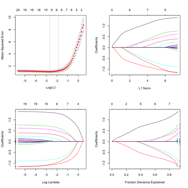
- Glmnet Vignette. It tries to minimize [math]\displaystyle{ RSS(\beta) + \lambda [(1-\alpha)\|\beta\|_2^2/2 + \alpha \|\beta\|_1] }[/math]. The elastic-net penalty is controlled by [math]\displaystyle{ \alpha }[/math], and bridge the gap between lasso ([math]\displaystyle{ \alpha = 1 }[/math]) and ridge ([math]\displaystyle{ \alpha = 0 }[/math]). Following is a CV curve (adaptive lasso) using the example from glmnet(). Two vertical lines are indicated: left one is lambda.min (that gives minimum mean cross-validated error) and right one is lambda.1se (the most regularized model such that error is within one standard error of the minimum). For the tuning parameter [math]\displaystyle{ \lambda }[/math],
- The larger the [math]\displaystyle{ \lambda }[/math], more coefficients are becoming zeros (think about coefficient path plots) and thus the simpler (more regularized) the model.
- If [math]\displaystyle{ \lambda }[/math] becomes zero, it reduces to the regular regression and if [math]\displaystyle{ \lambda }[/math] becomes infinity, the coefficients become zeros.
- In terms of the bias-variance tradeoff, the larger the [math]\displaystyle{ \lambda }[/math], the higher the bias and the lower the variance of the coefficient estimators.
- Video by Trevor Hastie
File:Glmnetplot.svg File:Glmnet path.svg File:Glmnet l1norm.svg
set.seed(1010)
n=1000;p=100
nzc=trunc(p/10)
x=matrix(rnorm(n*p),n,p)
beta=rnorm(nzc)
fx= x[,seq(nzc)] %*% beta
eps=rnorm(n)*5
y=drop(fx+eps)
px=exp(fx)
px=px/(1+px)
ly=rbinom(n=length(px),prob=px,size=1)

## Full lasso
library(doParallel)
registerDoParallel(cores = 2)
set.seed(999)
cv.full <- cv.glmnet(x, ly, family='binomial', alpha=1, parallel=TRUE)
plot(cv.full)  # cross-validation curve and two lambda's
plot(glmnet(x, ly, family='binomial', alpha=1), xvar="lambda", label=TRUE) # coefficient path plot
plot(glmnet(x, ly, family='binomial', alpha=1))  # L1 norm plot
log(cv.full$lambda.min) # -4.546394
log(cv.full$lambda.1se) # -3.61605
sum(coef(cv.full, s=cv.full$lambda.min) != 0) # 44

## Ridge Regression to create the Adaptive Weights Vector
set.seed(999)
cv.ridge <- cv.glmnet(x, ly, family='binomial', alpha=0, parallel=TRUE)
wt <- 1/abs(matrix(coef(cv.ridge, s=cv.ridge$lambda.min)
                   [, 1][2:(ncol(x)+1)] ))^1 ## Using gamma = 1, exclude intercept
## Adaptive Lasso using the 'penalty.factor' argument
set.seed(999)
cv.lasso <- cv.glmnet(x, ly, family='binomial', alpha=1, parallel=TRUE,
                      penalty.factor=wt)
# defautl type.measure="deviance" for logistic regression
plot(cv.lasso)
log(cv.lasso$lambda.min) # -2.995375
log(cv.lasso$lambda.1se) # -0.7625655
sum(coef(cv.lasso, s=cv.lasso$lambda.min) != 0) # 34
- cv.glmnet() has a logical parameter parallel which is useful if a cluster or cores have been previously allocated
- Ridge regression and the LASSO
- Standard error/Confidence interval
- Standard Errors in GLMNET and Confidence intervals for Ridge regression
- Why SEs are not meaningful and are usually not provided in penalized regression?
- Hint: standard errors are not very meaningful for strongly biased estimates such as arise from penalized estimation methods.
- Penalized estimation is a procedure that reduces the variance of estimators by introducing substantial bias.
- The bias of each estimator is therefore a major component of its mean squared error, whereas its variance may contribute only a small part.
- Any bootstrap-based calculations can only give an assessment of the variance of the estimates.
- Reliable estimates of the bias are only available if reliable unbiased estimates are available, which is typically not the case in situations in which penalized estimates are used.
- Hottest glmnet questions from stackexchange.
- Standard errors for lasso prediction. There might not be a consensus on a statistically valid method of calculating standard errors for the lasso predictions.
- Code for Adaptive-Lasso for Cox's proportional hazards model by Zhang & Lu (2007). This can compute the SE of estimates. The weights are originally based on the maximizers of the log partial likelihood. However, the beta may not be estimable in cases such as high-dimensional gene data, or the beta may be unstable if strong collinearity exists among covariates. In such cases, robust estimators such as ridge regression estimators would be used to determine the weights.
- Some issues:
- With group of highly correlated features, Lasso tends to select amongst them arbitrarily.
- Often empirically ridge has better predictive performance than lasso but lasso leads to sparser solution
- Elastic-net (Zou & Hastie '05) aims to address these issues: hybrid between Lasso and ridge regression, uses L1 and L2 penalties.
- Gradient-Free Optimization for GLMNET Parameters
- Outlier detection and robust variable selection via the penalized weighted LAD-LASSO method Jiang 2020
- LASSO REGRESSION (HOME MADE)
- Course notes on Optimization for Machine Learning
- High dimensional data analysis course by P. Breheny
- How to calculate R Squared value for Lasso regression using glmnet in R
- Getting AIC/BIC/Likelihood from GLMNet, AIC comparison in glmnet.
- Specifying categorical predictors in glmnet() - an example. The new solution is to use the makeX() function; see the vignette.
Lambda [math]\displaystyle{ \lambda }[/math]
- A list of potential lambdas: see Linear Regression case. The λ sequence is determined by lambda.max and lambda.min.ratio.
- lambda.max is computed from the input x and y; it is the maximal value for lambda such that all the coefficients are zero. How does glmnet compute the maximal lambda value? & Choosing the range and grid density for regularization parameter in LASSO. However see the Random data example.
- lambda.min.ratio (default is ifelse(nobs<nvars,0.01,0.0001)) is the ratio of smallest value of the generated λ sequence (say lambda.min) to lambda.max.
- The program then generated nlambda values linear on the log scale from lambda.max down to lambda.min.
- The sequence of lambda does not change with different data partitions from running cv.glmnet().
- Avoid supplying a single value for lambda (for predictions after CV use predict() instead). Supply instead a decreasing sequence of lambda values. I'll get different coefficients when I use coef(cv.glmnet obj) and coef(glmnet obj). See the complete code on gist.
cvfit <- cv.glmnet(x, y, family = "cox", nfolds=10)
fit <- glmnet(x, y, family = "cox", lambda = lambda)
coef.cv <- coef(cvfit, s = lambda)
coef.fit <- coef(fit)
length(coef.cv[coef.cv != 0]) # 31
length(coef.fit[coef.fit != 0]) # 30
all.equal(lambda, cvfit$lambda[40])  # TRUE
length(cvfit$lambda) # [1] 100
- Choosing hyper-parameters (α and λ) in penalized regression by Florian Privé
- lambda.min vs lambda.1se
- The lambda.1se represents the value of λ in the search that was simpler than the best model (lambda.min), but which has error within 1 standard error of the best model ( lambda.min < lambda.1se ). In other words, using the value of lambda.1se as the selected value for λ results in a model that is slightly simpler than the best model but which cannot be distinguished from the best model in terms of error given the uncertainty in the k-fold CV estimate of the error of the best model.
- lambda.1se can be checked by looking at the CV plot. The CV plot contains the SE of RMSE/Deviance and cv.glmnet object contains cvm and cvup elements. If we draw a horizontal line at cvup[i] where i is the index of the lambda.min, then the largest lambda satisfying cvm[j] <= cvup[i] will be lambda.1se. This can be seen on the example of Logistic Regression: family = "binomial".
- lambda.1se not being in one standard error of the error When we say 1 standard error, we are not talking about the standard error across the lambda's but the standard error across the folds for a given lambda. Suppose A=cvfit$cvsd[which(cv.lasso$lambda == cv.lasso$lambda.min)] is the sd at lambda.min and B=cvfit$cvm[which(cv.lasso$lambda == cv.lasso$lambda.min)] the minimum cross-validated MSE. If we draw a horizontal line at A+B, then the largest lambda less than the cross point (on x-axis) should be lambda.1se.
- The lambda.min option refers to value of λ at the lowest CV error. The error at this value of λ is the average of the errors over the k folds and hence this estimate of the error is uncertain.
- lambda.min, lambda.1se and Cross Validation in Lasso : Binomial Response, continuous reponse. It provides R code to calculate lambda.min and lambda.1se manually because cv.glmnet(, keep = TRUE) saves the folds information for us to reproduce the cross-validation results.
- https://www.rdocumentation.org/packages/glmnet/versions/2.0-10/topics/glmnet
- glmnetUtils: quality of life enhancements for elastic net regression with glmnet
- Mixing parameter: alpha=1 is the lasso penalty, and alpha=0 the ridge penalty and anything between 0–1 is Elastic net.
- RIdge regression uses Euclidean distance/L2-norm as the penalty. It won't remove any variables.
- Lasso uses L1-norm as the penalty. Some of the coefficients may be shrunk exactly to zero.
- In ridge regression and lasso, what is lambda?
- Lambda is a penalty coefficient. Large lambda will shrink the coefficients.
- cv.glment()$lambda.1se gives the most regularized model such that error is within one standard error of the minimum
- A deep dive into glmnet: penalty.factor, standardize, offset
- Lambda sequence is not affected by the "penalty.factor"
- How "penalty.factor" used by the objective function may need to be corrected
- A deep dive into glmnet: predict.glmnet
Optimal lambda for Cox model
See Regularization Paths for Cox’s Proportional Hazards Model via Coordinate Descent Simon 2011. We choose the λ value which maximizes [math]\displaystyle{ \hat{CV}(\lambda) }[/math].
- [math]\displaystyle{ \begin{align} \hat{CV}_{i}(\lambda) = l(\beta_{-i}(\lambda)) - l_{-i}(\beta_{-i}(\lambda)). \end{align} }[/math]
Our total goodness of fit estimate, [math]\displaystyle{ \hat{CV}(\lambda) }[/math], is the sum of all [math]\displaystyle{ \hat{CV}_{i}(\lambda). }[/math] By using the equation above – subtracting the log-partial likelihood evaluated on the non-left out data from that evaluated on the full data – we can make efficient use of the death times of the left out data in relation to the death times of all the data.
Get the partial likelihood of a Cox PH model with new data
Random data
- For random survival (response) data, glmnet easily returns 0 covariates by using lambda.min.
- For random binary or quantitative trait (response) data, it seems glmnet returns at least 1 covariate at lambda.min which is max(lambda). This seems contradicts the documentation which describes all coefficients are zero with max(lambda).
See the code here.
Multiple seeds in cross-validation
- Variablity in cv.glmnet results. From the cv.glmnet() reference manual: Note also that the results of cv.glmnet are random, since the folds are selected at random. Users can reduce this randomness by running cv.glmnet many times, and averaging the error curves.
MSEs <- NULL for (i in 1:100){ cv <- cv.glmnet(y, x, alpha=alpha, nfolds=k) MSEs <- cbind(MSEs, cv$cvm) } rownames(MSEs) <- cv$lambda lambda.min <- as.numeric(names(which.min(rowMeans(MSEs)))) - Stabilizing the lasso against cross-validation variability
- caret::trainControl(.., repeats, ...)
Cross Validated LASSO: What are its weaknesses?
Cross Validated LASSO with the glmnet package: What are its weaknesses?
At what lambda is each coefficient shrunk to 0
glmnet: at what lambda is each coefficient shrunk to 0?
Mixing parameter [math]\displaystyle{ \alpha }[/math]
cva.glmnet() from the glmnetUtils package to choose both the alpha and lambda parameters via cross-validation, following the approach described in the help page for cv.glmnet.
Underfittig, overfitting and relaxed lasso
- https://cran.r-project.org/web/packages/glmnet/vignettes/relax.pdf
- The Relaxed Lasso: A Better Way to Fit Linear and Logistic Models
- Overfitting: small lambda, lots of non-zero coefficients
- Underfitting: large lambda, not enough variables
- Relaxed Lasso by Nicolai Meinshausen
- Why is “relaxed lasso” different from standard lasso?
- https://web.stanford.edu/~hastie/TALKS/hastieJSM2017.pdf#page=13
- Stabilizing the lasso against cross-validation variability
Plots
library(glmnet)
data(QuickStartExample) # x is 100 x 20 matrix

cvfit = cv.glmnet(x, y)
fit = glmnet(x, y)

oldpar <- par(mfrow=c(2,2))
plot(cvfit) # mse vs log(lambda)
plot(fit) # coef vs L1 norm
plot(fit, xvar = "lambda", label = TRUE) # coef vs log(lambda)
plot(fit, xvar = "dev", label = TRUE) # coef vs Fraction Deviance Explained
par(oldpar)
print() method
?print.glmnet and ?print.cv.glmnet
Extract/compute deviance
deviance(fitted_glmnet_object)

coxnet.deviance(pred = NULL, y, x = 0, offset = NULL,
  weights = NULL, beta = NULL) # This calls a Fortran function loglike()
According to the source code, coxnet.deviance() returns 2 *(lsat-fit$flog).
coxnet.deviance() was used in assess.coxnet.R (CV, not intended for use by users) and buildPredmat.coxnetlist.R (CV).
See also Survival → glmnet.
coefplot: Plots Coefficients from Fitted Models
cv.glmnet and deviance
Usage
cv.glmnet(x, y, weights = NULL, offset = NULL, lambda = NULL,
  type.measure = c("default", "mse", "deviance", "class", "auc", "mae",
  "C"), nfolds = 10, foldid = NULL, alignment = c("lambda",
  "fraction"), grouped = TRUE, keep = FALSE, parallel = FALSE,
  gamma = c(0, 0.25, 0.5, 0.75, 1), relax = FALSE, trace.it = 0, ...)
type.measure parameter (loss to use for CV):
- default
- type.measure = deviance which uses squared-error for gaussian models (a.k.a type.measure="mse"), logistic and poisson regression (PS: for binary response data I found that type='class' gives a discontinuous CV curve while 'deviance' give a smooth CV curve), deviance formula for binomial model which is the same as the formula shown here and binomial glm case.
- type.measure = partial-likelihood for the Cox model (note that the y-axis from plot.cv.glmnet() gives deviance but the values are quite different from what deviace() gives from a non-CV modelling).
- mse or mae (mean absolute error) can be used by all models except the "cox"; they measure the deviation from the fitted mean to the response
- class applies to binomial and multinomial logistic regression only, and gives misclassification error.
- auc is for two-class logistic regression only, and gives area under the ROC curve. In order to calculate the AUC (which really needs a way to rank your test cases) glmnet needs at least 10 obs; see Calculate LOO-AUC values using glmnet.
- C is Harrel's concordance measure, only available for cox models
How to choose type.measure for binary response.
- Comparing AUC and classification loss for binary outcome in LASSO cross validation... For binary response, auc is thus preferable to class as a criterion for comparing models... But deviance is even better than auc... I can't say with certainty why the class criterion maintains fewer genes in the final model than does auc. I suspect that's because the class criterion is less sensitive to distinguishing among models.
- Why is accuracy not the best measure for assessing classification models? It discusses the imbalanced data. AUC is also not appropriate for imbalanced dataset.
grouped parameter
- This is an experimental argument, with default TRUE, and can be ignored by most users.
- For the "cox" family, grouped=TRUE obtains the CV partial likelihood for the Kth fold by subtraction; by subtracting the log partial likelihood evaluated on the full dataset from that evaluated on the on the (K-1)/K dataset. This makes more efficient use of risk sets. With grouped=FALSE the log partial likelihood is computed only on the Kth fold
- Gradient descent for the elastic net Cox-PH model
package deviance CV survival -2*fit$loglik[1] glmnet deviance(fit)
assess.glmnet(fit, newx, newy, family = "cox")
coxnet.deviance(x, y, beta)cv.glmnet(x, y, lambda, family="cox", nfolds, foldid)$cvm
which calls cv.glmnet.raw() (save lasso models for each CV)
which calls buildPredmat.coxnetlist(foldid) to create a matrix cvraw (eg 10x100)
and then calls cv.coxnet(foldid) (it creates weights of length 10 based on status and do cvraw/=weights)
and cvstats(foldid) which will calculate weighted mean of cvraw matrix for each lambda
and return the cvm vector; cvm[1]=sum(original cvraw[,1])/sum(weights)
Note: the document says the measure (cvm) is partial likelihood for survival data.
But cvraw calculation from buildPredmat.coxnetlist() shows the original/unweighted cvraw is CVPL.BhGLM measure.bh(fit, new.x, new.y) cv.bh(fit, nfolds=10, foldid, ncv)$measures[1]
which calls an internal function measure.cox(y.obj, lp) (lp is obtained from CV)
which calls bcoxph() [coxph()] using lp as the covariate and returns
deviance = -2 * ff$loglik[2] (a CV deviance)
cindex = summary(ff)$concordance[[1]] (a CV c-index)An example from the glmnet vignette The deviance value is the same from both survival::deviance() and glmnet::deviance(). But how about cv.glmnet()$cvm (partial-likelihood)?
library(glmnet)
library(survival)
library(tidyverse); library(magrittr)

data(CoxExample)
dim(x) # 1000 x 30
# I'll focus some lambdas based on one run of cv.glmnet()
set.seed(1); cvfit = cv.glmnet(x, y, family = "cox", lambda=c(10,2,1,.237,.016,.003))
rbind(cvfit$lambda, cvfit$cvm,
      deviance(glmnet(x, y, family = "cox", lambda=c(10, 2, 1, .237, .016, .003))))%>%
      set_rownames(c("lambda", "cvm", "deviance"))
               [,1]       [,2]       [,3]       [,4]       [,5]      [,6]
lambda     10.00000    2.00000    1.00000    0.23700    0.01600    0.0030
cvm        13.70484   13.70484   13.70484   13.70316   13.07713   13.1101
deviance 8177.16378 8177.16378 8177.16378 8177.16378 7707.53515 7697.3357

-2* coxph(Surv(y[,1], y[, 2]) ~ x)$loglik[1]
[1] 8177.164
coxph(Surv(y[,1], y[, 2]) ~ x)$loglik[1]
[1] -4088.582

# coxnet.deviance: compute the deviance (-2 log partial likelihood) for right-censored survival data
fit1 = glmnet(x, y, family = "cox", lambda=.016)
coxnet.deviance(x=x, y=y, beta=fit1$coef)
# [1] 8177.164
fit2 = glmnet(x, y, family = "cox", lambda=.003)
coxnet.deviance(x=x, y=y, beta=fit2$coef)
# [1] 8177.164

# assess.glmnet
assess.glmnet(fit1, newx=x, newy=y)
# $deviance
# [1] 7707.444
# attr(,"measure")
# [1] "Partial Likelihood Deviance"
#
# $C
# [1] 0.7331241
# attr(,"measure")
# [1] "C-index"

assess.glmnet(fit2, newx=x, newy=y)
# $deviance
# [1] 7697.314
# attr(,"measure")
# [1] "Partial Likelihood Deviance"
#
# $C
# [1] 0.7342417
# attr(,"measure")
# [1] "C-index"
What deviance is glmnet using
What deviance is glmnet using to compare values of 𝜆?
No need for glmnet if we have run cv.glmnet
https://stats.stackexchange.com/a/77549 Do not supply a single value for lambda. Supply instead a decreasing sequence of lambda values. glmnet relies on its warms starts for speed, and its often faster to fit a whole path than compute a single fit.
Exact definition of Deviance measure in glmnet package, with CV
- Exact definition of Deviance measure in glmnet package, with crossvalidation?
- https://glmnet.stanford.edu/reference/deviance.glmnet.html
cv.glmnet in cox model
Note: the CV result may changes unless we fix the random seed.
Note that the y-axis on the plot depends on the type.measure parameter. It is not the objective function used to find the estimator. For survival data, the y-axis is (residual) deviance (-2*loglikelihood, or RSS in linear regression case) [so the optimal lambda should give a minimal deviance value].
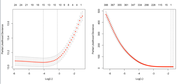
It is not always partial likelihood device has a largest value at a large lambda. In the following two plots, the first one is from the glmnet vignette and the 2nd one is from the coxnet vignette. The survival data are not sparse in both examples.
Sparse data
library(glmnet); library(survival)
n = 100; p <- 1000
beta1 = 2; beta2 = -1; beta3 =1; beta4 = -2
lambdaT = .002 # baseline hazard
lambdaC = .004  # hazard of censoring
set.seed(1234)
x1 = rnorm(n)
x2 = rnorm(n)
x3 <- rnorm(n)
x4 <- rnorm(n)
# true event time
T = Vectorize(rweibull)(n=1, shape=1, scale=lambdaT*exp(-beta1*x1-beta2*x2-beta3*x3-beta4*x4))
C = rweibull(n, shape=1, scale=lambdaC)   #censoring time
time = pmin(T,C)  #observed time is min of censored and true
event = time==T   # set to 1 if event is observed
cox <- coxph(Surv(time, event)~ x1 + x2 + x3 + x4); cox
-2*cox$loglik[2] # deviance [1] 301.7461
summary(cox)$concordance[1]  # 0.9006085

# create a sparse matrix
X <- cbind(x1, x2, x3, x4, matrix(rnorm(n*(p-4)), nr=n))
colnames(X) <- paste0("x", 1:p)
# X <- data.frame(X)
y <- Surv(time, event)
set.seed(1234)
nfold <- 10
foldid <- sample(rep(seq(nfold), length = n))
cvfit <- cv.glmnet(X, y, family = "cox", foldid = foldid)
plot(cvfit)
plot(cvfit$lambda, log = "y")
assess.glmnet(cvfit, newx=X, newy = y, family="cox") # return deviance 361.4619 and C 0.897421
            # Question: what lambda has been used?
            # Ans: assess.glmnet() calls predict.cv.glmnet() which by default uses s = "lambda.1se"

fit <- glmnet(X, y, family = "cox", lambda = cvfit$lambda.min)
assess.glmnet(fit, newx=X, newy = y, family="cox") # deviance 308.3646 and C 0.9382788
cvfit$cvm[cvfit$lambda == cvfit$lambda.min]
# [1] 7.959283

fit <- glmnet(X, y, family = "cox", lambda = cvfit$lambda.1se)
assess.glmnet(fit, newx=X, newy = y, family="cox") # deviance  361.4786 and C 0.897421
deviance(fit)
# [1] 361.4786

fit <- glmnet(X, y, family = "cox", lambda = 1e-3)
assess.glmnet(fit, newx=X, newy = y, family="cox") # deviance 13.33405 and C 1

fit <- glmnet(X, y, family = "cox", lambda = 1e-8)
assess.glmnet(fit, newx=X, newy = y, family="cox") # deviance 457.3695 and C .5

fit <- glmnet(cbind(x1,x2,x3,x4), y, family = "cox", lambda = 1e-8)
assess.glmnet(fit, newx=X, newy = y, family="cox")
# Error in h(simpleError(msg, call)) :
#  error in evaluating the argument 'x' in selecting a method for function 'as.matrix': Cholmod error
#  'X and/or Y have wrong dimensions' at file ../MatrixOps/cholmod_sdmult.c, line 90
deviance(fit) # [1] 301.7462

library(BhGLM)
X2 <- data.frame(X)
f1 = bmlasso(X2, y, family = "cox",  ss = c(.04, .5))
measure.bh(f1, X2, y)
# deviance   Cindex
#   303.39     0.90

o <- cv.bh(f1, foldid = foldid)
o$measures  # deviance and C
# deviance   Cindex
#  311.743    0.895
update() function
update() will update and (by default) re-fit a model. It does this by extracting the call stored in the object, updating the call and (by default) evaluating that call. Sometimes it is useful to call update with only one argument, for example if the data frame has been corrected.
It can be used in glmnet() object without a new implementation method.
- Linear regression
lm(y ~ x + z, data=myData)
lm(y ~ x + z, data=subset(myData, sex=="female"))
lm(y ~ x + z, data=subset(myData, age > 30))
- Lasso regression
R> fit <- glmnet(glmnet(X, y, family="cox", lambda=cvfit$lambda.min); fit
Call:  glmnet(x = X, y = y, family = "cox", lambda = cvfit$lambda.min)

  Df   %Dev Lambda
1 21 0.3002 0.1137

R> fit2 <- update(fit, subset = c(rep(T, 50), rep(F, 50)); fit2
Call:  glmnet(x = X[1:50, ], y = y[1:50], family = "cox", lambda = cvfit$lambda.min)

  Df   %Dev Lambda
1 24 0.4449 0.1137

R> fit3 <- update(fit, lambda=cvfit$lambda); fit3

Call:  glmnet(x = X, y = y, family = "cox", lambda = cvfit$lambda)

    Df    %Dev  Lambda
1    1 0.00000 0.34710
2    2 0.01597 0.33130
...
cv.glmnet and glmnet give different coefficients
glmnet: same lambda but different coefficients for glmnet() & cv.glmnet()
Number of nonzero in cv.glmnet plot is not monotonic in lambda
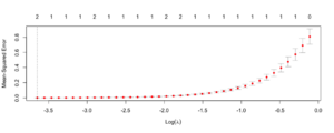
It is possible since this is based on CV? But if we use coef() to compute the nonzero coefficients for each lambda from the fitted model, it should be monotonic. Below is one case and the Cox regression example above is another case.
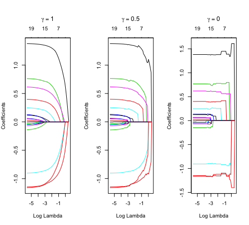
Relaxed fit and [math]\displaystyle{ \gamma }[/math] parameter
https://cran.r-project.org/web/packages/glmnet/vignettes/relax.pdf
Relaxed fit: Take a glmnet fitted object, and then for each lambda, refit the variables in the active set without any penalization.
Suppose the glmnet fitted linear predictor at [math]\displaystyle{ \lambda }[/math] is [math]\displaystyle{ \hat\eta_\lambda(x) }[/math] and the relaxed version is [math]\displaystyle{ \tilde\eta_\lambda(x) }[/math]. We also allow for shrinkage between the two:
- [math]\displaystyle{ \begin{align} \tilde \eta_{\lambda,\gamma}= \gamma\hat\eta_\lambda(x) + (1-\gamma)\tilde\eta_\lambda(x). \end{align} }[/math]
[math]\displaystyle{ \gamma\in[0,1] }[/math] is an additional tuning parameter which can be selected by cross validation.
The debiasing will potentially improve prediction performance, and CV will typically select a model with a smaller number of variables.
The default behavior of extractor functions like predict and coef, as well as plot will be to present results from the glmnet fit (not cv.glmnet), unless a value of [math]\displaystyle{ \gamma }[/math] is given different from the default value [math]\displaystyle{ \gamma=1 }[/math].
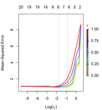
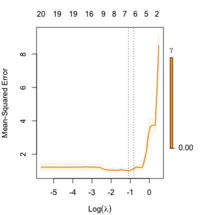
Question: how does cv.glmnet() select [math]\displaystyle{ \gamma }[/math] parameter? Ans: it depends on the parameter type.measure in cv.glmnet.
library(glmnet)
data(QuickStartExample)
fitr=glmnet(x,y, relax=TRUE)
set.seed(1)
cfitr=cv.glmnet(x,y,relax=TRUE)
c(fitr$lambda.min, fitr$lambda.1se)
# [1] 0.08307327 0.15932708
str(cfitr$relaxed)
plot(cfitr),oldpar <- par(mfrow=c(1,3), mar = c(5,4,6,2))
plot(fitr, main = expression(gamma == 1))
plot(fitr,gamma=0.5, main = expression(gamma == .5))
plot(fitr,gamma=0, main = expression(gamma == 0))
par(oldpar)
Special cases: - [math]\displaystyle{ \gamma=1 }[/math]: only regularized fit, no relaxed fit.
- [math]\displaystyle{ \gamma=0 }[/math]: only relaxed fit; a faster version of forward stepwise regression.
set.seed(1)
cfitr2=cv.glmnet(x,y,gamma=0,relax=TRUE)
  # default gamma = c(0, 0.25, 0.5, 0.75, 1)
plot(cfitr2)
c(cfitr2$lambda.min, cfitr2$lambda.1se)
# [1] 0.08307327 0.15932708
str(cfitr2$relaxed)
Computation time
beta1 = 2; beta2 = -1
lambdaT = .002 # baseline hazard
lambdaC = .004  # hazard of censoring
set.seed(1234)
x1 = rnorm(n)
x2 = rnorm(n)
# true event time
T = Vectorize(rweibull)(n=1, shape=1, scale=lambdaT*exp(-beta1*x1-beta2*x2))
# No censoring
event2 <- rep(1, length(T))

system.time(fit <- cv.glmnet(x, Surv(T,event2), family = 'cox'))
#    user  system elapsed
#   4.701   0.016   4.721
system.time(fitr <- cv.glmnet(x, Surv(T,event2), family = 'cox', relax= TRUE))
#    user  system elapsed
# 161.002   0.382 161.573
predict() and coef() methods
?predict.glmnet OR ?coef.glmnet OR ?coef.relaxed. Similar to other predict methods, this functions predicts fitted values, logits, coefficients and more from a fitted "glmnet" object.
## S3 method for class 'glmnet'
predict(object, newx, s = NULL, type = c("link",
  "response", "coefficients", "nonzero", "class"), exact = FALSE,
  newoffset, ...)

## S3 method for class 'relaxed'
predict(object, newx, s = NULL, gamma = 1,
  type = c("link", "response", "coefficients", "nonzero", "class"),
  exact = FALSE, newoffset, ...)
## S3 method for class 'glmnet'
coef(object, s = NULL, exact = FALSE, ...)
?predict.cv.glmnet OR ?coef.cv.glmnet OR ?coef.cv.relaxed. This function makes predictions from a cross-validated glmnet model, using the stored "glmnet.fit" object, and the optimal value chosen for lambda (and gamma for a 'relaxed' fit).
## S3 method for class 'cv.glmnet'
predict(object, newx, s = c("lambda.1se",
  "lambda.min"), ...)

## S3 method for class 'cv.relaxed'
predict(object, newx, s = c("lambda.1se",
  "lambda.min"), gamma = c("gamma.1se", "gamma.min"), ...)
AUC
- Validating AUC values in R's GLMNET package.
fit = cv.glmnet(x = data, y = label, family = 'binomial', alpha=1, type.measure = "auc")
pred = predict(fit, newx = data, type = 'response',s ="lambda.min")
auc(label,pred)
- Computing the auc for test data using cv.glmnet
Cindex
https://www.rdocumentation.org/packages/glmnet/versions/3.0-2/topics/Cindex
Usage:
Cindex(pred, y, weights = rep(1, nrow(y)))
assess.glmnet
https://www.rdocumentation.org/packages/glmnet/versions/3.0-2/topics/assess.glmnet
Usage:
assess.glmnet(object, newx = NULL, newy, weights = NULL,
  family = c("gaussian", "binomial", "poisson", "multinomial", "cox",
  "mgaussian"), ...)
confusion.glmnet(object, newx = NULL, newy, family = c("binomial",
  "multinomial"), ...)

roc.glmnet(object, newx = NULL, newy, ...)
Variable importance
- Variable importance from GLMNET; (coef from glmnet) * (SD of variables) = standardized coef
- glmnet - variable importance? Note not sure if caret considers scales of variables.
- A plot of showing the importance of variables by ranking the variables in a heatmap Gerstung 2015. The plot looks nice but the way of ranking variables seems not right (not based on the optimal lambda).
- Random forest
- glmnet variable importance | `vip` vs `varImp`
R-square/R2 and dev.ratio
- How to calculate 𝑅2 for LASSO (glmnet). Use cvfit$glmnet.fit$dev.ratio. According to ?glmnet, dev.ratio is the fraction of (null) deviance explained (for "elnet", this is the R-square).
- How to calculate R Squared value for Lasso regression using glmnet in R
- Coefficient of determination from wikipedia. R2 is the proportion of the variation in the dependent variable that is predictable from the independent variable(s).
- What is the main difference between multiple R-squared and correlation coefficient? It provides 4 ways (same value) to calculate R2 for multiple regression (not glmnet).
fm <- lm(Y ~ X1 + X2) # regression of Y on X1 and X2
fm_null <- lm(Y ~ 1)  # null model

# Method 1: definition
var(fitted(fm)) / var(Y) # ratio of variances
# Method 2
cor(fitted(fm), Y)^2 # squared correlation
# Method 3
summary(fm)$r.squared # multiple R squared
# Method 4
1 - deviance(fm) / deviance(fm_null)  # improvement in residual sum of squares
- %Dev is R2 in linear regression case. How to calculate R Squared value for Lasso regression using glmnet in R, How to calculate 𝑅2 for LASSO (glmnet)
library(glmnet)
data(QuickStartExample)
x <- QuickStartExample$x
y <- QuickStartExample$y
dim(x)
# [1] 100  20

fit2 <- lm(y~x)
summary(fit2)
# Multiple R-squared:  0.9132,    Adjusted R-squared:  0.8912

glmnet(x, y)
#    Df  %Dev  Lambda
# 1   0  0.00 1.63100
# 2   2  5.53 1.48600
# 3   2 14.59 1.35400
# ...
# 64 20 91.31 0.00464
# 65 20 91.32 0.00423
# 66 20 91.32 0.00386
# 67 20 91.32 0.00351
- An example to get R2 (deviance) from glmnet. %DEV or cv.glmnet()$glmnet.fit$dev.ratio is fraction of (null) deviance explained. ?deviance.glmnet
set.seed(1010)
n=1000;p=100
nzc=trunc(p/10)
x=matrix(rnorm(n*p),n,p)
beta=rnorm(nzc)
fx= x[,seq(nzc)] %*% beta
eps=rnorm(n)*5
y=drop(fx+eps)

set.seed(999)
cvfit <- cv.glmnet(x, y)
cvfit
# Measure: Mean-Squared Error
#     Lambda Index Measure     SE Nonzero
# min 0.2096    24   24.32 0.8105      21
# 1se 0.3663    18   24.93 0.8808      12
cvfit$cvm[cvfit$lambda == cvfit$lambda.min]
# 24.3218   <- mean cross-validated error
cvfit$glmnet.fit
#    Df  %Dev  Lambda
# 1   0  0.00 1.78100
# 2   1  1.72 1.62300
# 23 19 25.40 0.23000
# 24 21 25.96 0.20960  <- Same as glmnet() result   -----------------------------+
# 25 21 26.44 0.19100                                                            |
# ...                                                                            |
cvfit$glmnet.fit$dev.ratio[cvfit$lambda == cvfit$lambda.min]                     |
# [1] 0.2596395   dev.ratio=1-dev/nulldev. ?deviance.glmnet                      |
                                                                                 |
fit <- glmnet(x, y, lambda=cvfit$lambda.min); fit                                |
#   Df  %Dev Lambda                                                              |
# 1 21 25.96 0.2096    <---------------------------------------------------------+
predict.lasso <- predict(fit, newx=x, s="lambda.min", type = 'response')[,1]     |
                                                                                 |
1 - deviance(fit)/deviance(lm(y~1))                                              |
# [1] 0.2596395   <- Same as glmnet()  ------------------------------------------+
deviance(lm(y~1))  # Same as sum((y-mean(y))**2)
deviance(fit)      # Same as sum((y-predict.lasso)**2)
cor(predict.lasso, y)^2
# [1] 0.2714228   <- Not the same as glmnet()
var(predict.lasso) / var(y)
# [1] 0.1701002   <- Not the same as glmnet()
ridge regression and multicollinear
https://en.wikipedia.org/wiki/Ridge_regression. Ridge regression is a method of estimating the coefficients of multiple-regression models in scenarios where linearly independent variables are highly correlated.
# example from SGL package set.seed(1) n = 50; p = 100; size.groups = 10 X = matrix(rnorm(n * p), ncol = p, nrow = n) beta = (-2:2) y = X[,1:5] %*% beta + 0.1*rnorm(n) data = list(x = X, y = y) cvfit <- cv.glmnet(X, y, alpha = 0) plot(cvfit) o <- coef(cvfit, lambda = cvfit$lambda.min) %>% drop() sum(o != 0) # [1] 101. # Too biased. o[1:10] # (Intercept) V1 V2 V3 V4 # -3.269401e-01 -2.253226e-36 -8.900799e-37 5.198885e-37 1.311976e-36 # V5 V6 V7 V8 V9 # 1.873125e-36 1.582532e-37 2.085781e-37 4.732839e-37 2.997614e-37 y_predicted <- predict(cvfit, s = cvfit$lambda.min, newx = X) # Sum of Squares Total and Error sst <- sum((y - mean(y))^2) sse <- sum((y_predicted - y)^2) # R squared rsq <- 1 - sse / sst rsq # 0.46 library(SGL) # sparse group lasso set.seed(1) index <- ceiling(1:p / size.groups) cvFit = cvSGL(data, index, type = "linear", alpha=.95) # this alpha is the default plot(cvFit) cvFit$fit$beta[, 20] # 20th lambda gives smallest negative log likelihood # identify correct predictors # [1] -10.942712 -6.167799 0.000000 6.595406 14.442019 0.000000 ... set.seed(1) cvFit2 = cvSGL(data, index, type = "linear", alpha=0) plot(cvFit2) cvFit2$fit$beta[, 20] # [1] -10.8417371 -6.5251240 0.2476438 6.7223001 14.1605263 0.2149542 # [7] 0.2481450 0.1404282 0.1799818 0.3784596 0.0000000 0.0000000 ...- Tikhonov regularization (ridge regression). It was used to handle ill-posed/overfitting situation. Ridge regression shrinks the coefficients by a uniform factor of [math]\displaystyle{ {\displaystyle (1+N\lambda )^{-1}}{\displaystyle (1+N\lambda )^{-1}} }[/math] and does not set any coefficients to zero.
- cvSGL
- How and when: ridge regression with glmnet. On training data, ridge regression fits less well than the OLS but the parameter estimate is more stable. So it does better in prediction because it is less sensitive to extreme variance in the data such as outliers.
Filtering variables
See its vignette.
One might think that unsupervised filtering using just x before fitting the model is fair game, and perhaps need not be accounted for in cross-validation. This is an interesting issue, and one can argue that there could be some bias if it was not accounted for. But filtering using x and y definitely introduces potential bias. However, it can still give good results, as long as it it correctly accounted for when running CV.
Graphical lasso
- Wikipedia
- Google scholar cited by 5k.
- Sparse inverse covariance estimation with the graphical lasso Friedman 2008. Number 3 of highly cited articles.
Group lasso
- BhGLM on github, Gsslasso Cox: a Bayesian hierarchical model for predicting survival and detecting associated genes by incorporating pathway information 2019
- grplasso package. Why use group lasso instead of lasso? Already for the special case in linear regression when not only continuous but also categorical predictors (factors) are present, the lasso solution is not satisfactory as it only selects individual dummy variables instead of whole factors. Moreover, the lasso solution depends on how the dummy variables are encoded. Choosing different contrasts for a categorical predictor will produce different solutions in general.
- gglasso: Group Lasso Penalized Learning Using a Unified BMD Algorithm. Using LASSO in R with categorical variables
- SGL
- Group Lasso implementation following the scikit-learn API with nice documentation
- Seagull: lasso, group lasso and sparse-group lasso regularization for linear regression models via proximal gradient descent. CRAN.
- MSGLasso
- sgPLS, paper Liquet 2016
- pcLasso: Principal Components Lasso package
- pclasso paper, slides, Blog
- Each feature must be assigned to a group
- It allows to assign each feature to groups (including overlapping).
library(pcLasso)

set.seed(1)
n = 50; p = 100; size.groups = 10
index <- ceiling(1:p / size.groups)
X = matrix(rnorm(n * p), ncol = p, nrow = n)
beta = (-2:2)
y = X[,1:5] %*% beta + 0.1*rnorm(n)

groups <- vector("list", 3)
for (k in 1:2) {
    groups[[k]] <- 5 * (k-1) + 1:5
}
groups[[3]] <- 11:p
cvfit <- cv.pcLasso(X, y, ratio = 0.8, groups = groups)
plot(cvfit)

pred.pclasso <- predict(cvfit, xnew = X, s = "lambda.min")
mean((y-pred.pclasso)^2)  #  [1] 1.956387

library(SGL)
index <- ceiling(1:p / size.groups)
data = list(x = X, y = y)
set.seed(1)
cvFit = cvSGL(data, index, type = "linear")
Fit = SGL(data, index, type = "linear")
  # 1. SGL() uses a different set of lambdas than cvSGL() does (WHY)
  #    After looking at cvFit$lambdas; Fit$lambdas
  #    I should pick the last lambda; the smallest
  # 2. predictSGL() source code shows Fit$X.transform$X.means
  #    and Fit$X.transform$X.scale should be applied to the new data
  #    before it calls X %*% x$beta[, lam] + intercept
  # 3. The returned values of predictSGL() depends on the response type
  #    (linear, logit or cox).
  #    For linear, it returns eta = X %*% x$beta[, lam] + intercept
  #    For logit, it returns exp(eta)/(1 + exp(eta))
  #    For cox, it returns exp(eta)
pred.SGL <- predictSGL(Fit, X, length(Fit$lambdas))
mean((y-pred.SGL)^2)    # [1] 0.146027
# Coefficients
Fit$beta[, 20]
Fit$intercept

library(ggplot2)
library(tidyr)
dat <- tibble(y=y, SGL=pred.SGL, pclasso=pred.pclasso) %>% gather("method", "predict", 2:3)

ggplot(dat, aes(x=y, y=predict, color=method)) + geom_point() + geom_abline(slope=1)
- Spike-and-slab regression
- Gsslasso Cox: A Bayesian Hierarchical Model for Predicting Survival and Detecting Associated Genes by Incorporating Pathway Information, Tang et al., 2019
- Spike-and-Slab Group Lassos for Grouped Regression and Sparse Generalized Additive Models Bai 2020
- Spike-and-slab type variable selection in the Cox proportional hazards model for high-dimensional features Wu 2021
- Fast Sparse-Group Lasso Method for Multi-response Cox Model with Applications to UK Biobank Li 2020
- Adaptive group-regularized logistic elastic net regression 2021. gren package in CRAN.
- Lasso, Group Lasso, and Exclusive Lasso
- Peel learning for pathway-related outcome prediction & Python code Li 2021
- Accounting for grouped predictor variables or pathways in high-dimensional penalized Cox regression models 2020.
Minimax concave penalty (MCP)
- The minimax concave penalty (MCP)
- High-dimensional data anlaysis by Patrick Breheny
- grpregOverlap and grpreg
- ncvreg package by Patrick Breheny. It is an R package for fitting regularization paths for linear regression, GLM, and Cox regression models using lasso or nonconvex penalties, in particular the minimax concave penalty (MCP) and smoothly clipped absolute deviation (SCAD) penalty, with options for additional L2 penalties (the “elastic net” idea).
- glmgraph
penalty.factor
The is available in glmnet() but not in cv.glmnet().
Collinearity
- Collinearity from Applied Statistics with R by David Dalpiaz
- Collinearity: a review of methods to deal with it and a simulation study evaluating their performance 2012
categorical covariates, multi-collinearity/multicollinearity, contrasts()
- Group lasso
- Can glmnet logistic regression directly handle factor (categorical) variables without needing dummy variables?
x_train <- model.matrix( ~ .-1, factor(x)) # affect encoding for the 1st level; see ?formula
cvfit = cv.glmnet(x=x_train, y=y, intercept=FALSE)
coef(cvfit, s="lambda.min") # still contains intercept but it is 0
- GLM vs Lasso vs SGL
library(glmnet) library(SGL) set.seed(1010) n=1000;p=100 nzc=trunc(p/10) x=matrix(rnorm(n*p),n,p) beta=rnorm(nzc) tumortype <- sample(c(1:4), size = n, replace = TRUE) fx= x[,seq(nzc)] %*% beta + .5*tumortype eps=rnorm(n)*5 y=drop(fx+eps) if (FALSE) { # binary response based on the logistic model px=exp(fx) px=px/(1+px) ly=rbinom(n=length(px),prob=px,size=1) } # glm. Assume we know the true variables. df <- cbind(data.frame(x[, 1:10]), tumortype, y) colnames(df) <- c(paste0("x", 1:10), "tumortype", "y") mod <- glm(y ~ ., data = df) broom::tidy(mod) # summary(mod) pred.glm <- predict(mod, newdata = df) mean((y-pred.glm)^2) # 23.32704 # lasso 1. tumortype is continuous X <- cbind(x, tumortype) set.seed(1234) fit.lasso <- cv.glmnet(X, y, alpha=1) predict.lasso1 <- predict(fit.lasso, newx=X, s="lambda.min", type = 'response')[,1] coef.lasso1 <- coef(fit.lasso)[,1] sum(coef.lasso1 != 0) # 11 unname(which(coef.lasso1 != 0)) # [1] 1 2 3 4 5 7 8 9 10 71 102 mean((y-predict.lasso1)^2) # 23.2942 # lasso 2. tumortype is categorical, intercept = FALSE X <- cbind(x, model.matrix( ~ .-1, data.frame(factor(tumortype)))) dim(X) # 104 columns set.seed(1234) fit.lasso2 <- cv.glmnet(X, y, alpha=1, intercept = FALSE) predict.lasso2 <- predict(fit.lasso2, newx=X, s="lambda.min", type = 'response')[,1] coef.lasso2 <- coef(fit.lasso2)[,1] length(coef.lasso2) # 105 sum(coef.lasso2 != 0) # 12 unname(which(coef.lasso2 != 0)) # [1] 2 3 4 5 7 8 9 10 71 103 104 105 mean((y-predict.lasso2)^2) # 23.3353 # lasso 3. tumortype is categorical, intercept = TRUE set.seed(1234) fit.lasso3 <- cv.glmnet(X, y, alpha=1) predict.lasso3 <- predict(fit.lasso3, newx=X, s="lambda.min", type = 'response')[,1] coef.lasso3 <- coef(fit.lasso3)[,1] length(coef.lasso3) # 105 sum(coef.lasso3 != 0) # 11 unname(which(coef.lasso3 != 0)) # [1] 1 2 3 4 5 7 8 9 10 71 102 mean((y-predict.lasso3)^2) # 23.16397 # SGL set.seed(1234) index <- c(1:p, rep(p+1, nlevels(factor(tumortype)))) data <- list(x=X, y=y) cvFit = cvSGL(data, index, type = "linear", alpha=.95) # this alpha is the default # this takes a longer time plot(cvFit) i <- which.min(cvFit$lldiff); i # 15 Fit = SGL(data, index, type = "linear", lambdas = cvFit$lambdas) sum(Fit$beta[, i] != 0) # 28 pred.SGL <- predictSGL(Fit, X, i) mean((y-pred.SGL)^2) # 23.33841 which(Fit$beta[, i] != 0) # [1] 1 2 3 4 6 7 8 9 10 12 21 23 29 35 37 40 45 # [18] 53 60 62 68 70 85 86 101 102 103 104 # Plot. A mess unless n is small dat <- tibble(y=y, glm=pred.glm, lasso1=predict.lasso1, lasso2=predict.lasso2, SGL=pred.SGL) %>% pivot_longer(-y, names_to="method", values_to="predict") ggplot(dat, aes(x=y, y=predict, color=method)) + geom_point() + geom_abline(slope=1) - How to include all levels of a factor variable in a model matrix in R - model.matrix, Changing the column names for model.matrix output
- Original post All Levels of a Factor in a Model Matrix in R. caret::dummyVars()
- ?dummyVars
- How does glmnet's standardize argument handle dummy variables?
Adaptive lasso and weights
Oracle property and adaptive lasso
- Variable Selection via Nonconcave Penalized Likelihood and Its Oracle Properties, Fan & Li (2001) JASA
- Adaptive Lasso: What it is and how to implement in R. Adaptive lasso weeks to minimize [math]\displaystyle{ RSS(\beta) + \lambda \sum_1^p \hat{\omega}_j |\beta_j| }[/math] where [math]\displaystyle{ \lambda }[/math] is the tuning parameter, [math]\displaystyle{ \hat{\omega}_j = \frac{1}{(|\hat{\beta}_j^{ini}|)^\gamma} }[/math] is the adaptive weights vector and [math]\displaystyle{ \hat{\beta}_j^{ini} }[/math] is an initial estimate of the coefficients obtained through ridge regression. Adaptive Lasso ends up penalizing more those coefficients with lower initial estimates. [math]\displaystyle{ \gamma }[/math] is a positive constant for adjustment of the adaptive weight vector, and the authors suggest the possible values of 0.5, 1 and 2.
- When n goes to infinity, [math]\displaystyle{ \hat{\omega}_j |\beta_j| }[/math] converges to [math]\displaystyle{ I(\beta_j \neq 0) }[/math]. So the adaptive Lasso procedure can be regarded as an automatic implementation of best-subset selection in some asymptotic sense.
- What is the oracle property of an estimator? An oracle estimator must be consistent in 1) variable selection and 2) consistent parameter estimation.
- Oracle property: Oracle property is a name given to techniques for estimating the regression parameters in the models fitted to high-dimensional data which have the property that they can correctly select the nonzero coefficients with the probability converging to one and that the estimators of nonzero coefficients are asymptotically normal with the identical means and covariances that they would have if the zero coefficients were known in advance that is the estimators are asymptotically as efficient as the ideal estimation assisted by an 'oracle' who knows which coefficients are nonzero.
- (Linear regression) The adaptive lasso and its oracle properties Zou (2006, JASA)
- (Cox model) Adaptive-LASSO for Cox's proportional hazard model by Zhang and Lu (2007, Biometrika)
- When the LASSO fails???. Adaptive lasso is used to demonstrate its usefulness.
- On the use of cross-validation for the calibration of the adaptive lasso Ballout 2023
Survival data
- The sum of errors term can be replaced with [math]\displaystyle{ -l(\beta, \gamma) }[/math], where [math]\displaystyle{ l(\cdot, \cdot) }[/math] stands for the log-likelihood function and [math]\displaystyle{ \gamma }[/math] for the intercept. See The lasso method for variable selection in the cox model 1997.
- Regularization Paths for Cox's Proportional Hazards Model via Coordinate Descent Noah Simon, Jerome H. Friedman, Trevor Hastie, Rob Tibshirani, 2011
- Cox regression: Estimation by Patrick Breheny
- Another implementation coxnet
- Gradient lasso for Cox proportional hazards model
- Prediction method. ?predict.cv.glmnet is not clear. ?coef.glmnet is more clear.
data(CoxExample)
dim(x) # 1000 x 30
ind.train <- 1:nrow(x)/2
cv.fit <- cv.glmnet(x[ind.train, ], y[ind.train, ], family="cox")
coef(cv.fit, s = "lambda.min")
    # 30 x 1, coef(...) is equivalent to predict(type="coefficients",...)
pr <- predict(cv.fit, x[-ind.train, ], type = "link", s = "lambda.min")
    # the default option for type is 'link' which gives the linear predictors for "cox" models.
pr2 <- x[-ind.train, ] %*% coef(cv.fit, s = "lambda.min")
all.equal(pr[, 1], pr2[, 1]) # [1] TRUE
class(pr) # [1] "matrix"
class(pr2) # [1] "dgeMatrix"
# we can also use predict() with glmnet object
pr22 <- predict(fit, x[-ind.train, ], type='link', s = cv.fit$lambda.min)
all.equal(pr[, 1], pr22[, 1]) # [1] TRUE

pr3 <- predict(cv.fit, x[-ind.train, ], type = "response", s = "lambda.min")
range(pr3)  # relative risk [1]  0.05310623 19.80143519
- Solving the Cox Proportional Hazards Model and Its Applications. Solving the Model by Coordinate Descent.
Logistic
- Warning of too few observations
cv.glmnet warnings for logit model (although binomial classes with more than 8 obs)?
1: In lognet(xd, is.sparse, ix, jx, y, weights, offset, alpha, nobs,  :
  one multinomial or binomial class has fewer than 8  observations; dangerous ground
Multi-response
Survival analysis on rare events using group-regularized multi-response Cox regression Li et al 2021
Weights on samples for unbalanced responses data for binary response
w1 <- rep(1, n.sample)
w1[bin == "Sensitive" <- sum(bin == "Resistant") / sum(bin == "Sensitive")
cv.glmnet(xx, yy, family = 'binomial', weights = w1)
Proportional matrix: family="binomial"
What does a proportional matrix look like for glmnet response variable in R? You can provide a matrix of proportion, 2nd column for success but this assumes the weight or n is same for all observations:
glmnet 4.0: family
glmnet v4.0: generalizing the family parameter
Timing
nvec <- c(100, 400)
pvec <- c(1000, 5000)
for(n in nvec)
  for(p in pvec) {
    nzc = trunc(p/10)  # 1/10 variables are non-zeros
    x = matrix(rnorm(n * p), n, p)
    beta = rnorm(nzc)
    fx = x[, seq(nzc)] %*% beta/3
    hx = exp(fx)
    ty = rexp(n, hx)
    tcens = rbinom(n = n, prob = 0.3, size = 1)  # censoring indicator
    y = cbind(time = ty, status = 1 - tcens)  # y=Surv(ty,1-tcens) with library(survival)
    foldid = sample(rep(seq(10), length = n))
    o <- system.time(fit1_cv <- cv.glmnet(x, y, family = "cox", foldid = foldid) )
    cat(sprintf("n=%1d, p=%5d, time=%8.3f\n", n, p, o['elapsed']))
}
Running on core i7 2.6GHz, macbook pro 2018. Unit is seconds.
p ∖ n 100 400 1000 5 58 5000 9 96 Xeon E5-2680 v4 @ 2.40GHz
p ∖ n 100 400 1000 7 98 5000 13 125 All interactions
How to make all interactions before using glmnet
Algorithm
warm start
- Why is my Rcpp code is much slower than glmnet's?
- Lasso: Algorithms by Patrick Breheny
Gradient descent
- Parameter: learning rate/alpha. If the steps are too large, gradient descent may never reach the local minimum, as displayed above. If the steps are too small, gradient descent will eventually reach the local minimum but it will take much too long to get there.
- Gradient Descent, Step-by-Step by StatQuest
- Gradient Descent: Explained!
- Gradient Descent Explained Simply with Examples
- Gradient descent for the elastic net Cox-PH model
- Gradient descent in R
Cyclical coordinate descent algorithm
- The glmnet algorithms use cyclical coordinate descent, which successively optimizes the objective function over each parameter with others fixed, and cycles repeatedly until convergence. See the An Introduction to glmnet vignettes
- A deep dive into glmnet: type.gaussian
- Coordinate descent
Quadratic programming
- Optimization and Mathematical Programming
- Optimization with R –Tips and Tricks
- Quadratic Programming with R
- Using quadratic programming to solve L1-norm regularization.
- The examples there pick up specified lambdas in order to compare the solutions from glmnet and quadratic programming and
- The examples still have n>p. If p>n, then it is impossible to compute the norm of the least squares solution. So it is difficult to get the shrinkage size and there is no way to reproduce glmnet solution using quadratic programming packages.
Other
- Ridge coefficient estimates do not match OLS estimates when lambda = 0. Adjust
- thresh - Convergence threshold for coordinate descent. Each inner coordinate-descent loop continues until the maximum change in the objective after any coefficient update is less than thresh times the null deviance. Defaults value is 1E-7.
- pmax - Limit the maximum number of variables ever to be nonzero
- dfmax - Limit the maximum number of variables in the model. Useful for very large nvars, if a partial path is desired.
- Make cv.glmnet select something between lambda.min and lambda.1se
- Difference Between Built-In Cross Validation Functions and Using Caret
Simulation study
- Stabilizing the lasso against cross-validation variability 2014
- Empirical extensions of the lasso penalty to reduce the false discovery rate in high-dimensional Cox regression models 2016
- Lab 3: Regularization procedures with glmnet
Feature selection
- Feature selection and survival modeling in The Cancer Genome Atlas Kim 2013.
- BOSO: A novel feature selection algorithm for linear regression with high-dimensional data 2022
- Feature-specific inference for penalized regression using local false discovery rates 2023
Release
- glmnet v4.1: regularized Cox models for (start, stop and stratified data]
- glmnet v4.0: generalizing the family parameter
Discussion
- https://stackoverflow.com/questions/tagged/glmnet
- https://stats.stackexchange.com/questions/tagged/glmnet
Prediction
- Comparison of pathway and gene-level models for cancer prognosis prediction Zheng, 2020
- Cancer prognosis prediction using somatic point mutation and copy number variation data: a comparison of gene-level and pathway-based models Zheng 2020
- CAncer bioMarker Prediction Pipeline (CAMPP)—A standardized framework for the analysis of quantitative biological data Terkelsen, 2020
- Comparison of likelihood penalization and variance decomposition approaches for clinical prediction models: A simulation study Lohmann 2023
- Compares the out-of-sample predictive performance of risk prediction models derived using the elastic net, with Lasso and ridge as special cases, and variance decomposition techniques, namely, incomplete principal component regression and incomplete partial least squares regression.
- Predictive performance was compared on measures of discrimination, calibration, and prediction error.
- Prediction models developed using penalization and variance decomposition approaches outperform models developed using ordinary maximum likelihood estimation, with penalization approaches being consistently superior over the variance decomposition approaches.
- Differences in performance were most pronounced on the calibration of the model.
- Code https://osf.io/gcjn6/
- discussion from Harrell
ROC
How to plot ROC-curve for logistic regression (LASSO) in R?
LASSO vs Least angle regression
- https://web.stanford.edu/~hastie/Papers/LARS/LeastAngle_2002.pdf
- Least Angle Regression, Forward Stagewise and the Lasso
- https://www.quora.com/What-is-Least-Angle-Regression-and-when-should-it-be-used
- A simple explanation of the Lasso and Least Angle Regression
- https://stats.stackexchange.com/questions/4663/least-angle-regression-vs-lasso
- https://cran.r-project.org/web/packages/lars/index.html
- How to use cv.lars()
test_lasso=lars(A,B)
test_lasso_cv=cv.lars(A,B)
bestfraction = test_lasso_cv$index[which.min(test_lasso_cv$cv)]
#Find Coefficients
coef.lasso = predict(test_lasso,A),s=bestfraction,type="coefficient",mode="fraction")
- Use of lars() function for LASSO
lasso.fit<-lars(x, y, type="lasso")
cv.lasso.fit<-cv.lars(x, y, K=10, index=seq(from=0, to=1, length=20))
yhat<-predict(lasso.fit, newx=x, s=0.368, type="fit", mode="fraction")
plot(y, yhat$fit)
abline(a=0, b=1)

coef(lasso.fit, s=0.526, mode="fraction")
yhat2<-predict(lasso.fit, newx=x, s=0.526, type="fit", mode="fraction")
- Why do Lars and Glmnet give different solutions for the Lasso problem?
LassoNet
caret
Tidymodels and tune
biglasso
biglasso: Extend Lasso Model Fitting to Big Data in R
snpnet
snpnet: Efficient Lasso Solver for Large-scale SNP Data
cornet: Elastic Net with Dichotomised Outcomes
- https://cran.r-project.org/web/packages/cornet/index.html
- Predicting dichotomised outcomes from high-dimensional data in biomedicine
- biomedical researchers often convert numerical to binary outcomes (loss of information) to conduct logistic regression (probabilistic interpretation).
- The proposed approach effectively combines binary with numerical outcomes to improve binary classification in high-dimensional settings.
Other methods, reviews
- Structured sparsity regularization for analyzing high-dimensional omics data Vinga 2021
- An efficient gene selection method for microarray data based on LASSO and BPSO
- A Tuning-free Robust and Efficient Approach to High-dimensional Regression
- Sparse sliced inverse regression for high dimensional data analysis Hilafu 2022


