Glmnet
Basic
- https://en.wikipedia.org/wiki/Lasso_(statistics). It has a discussion when two covariates are highly correlated. For example if gene [math]\displaystyle{ i }[/math] and gene [math]\displaystyle{ j }[/math] are identical, then the values of [math]\displaystyle{ \beta _{j} }[/math] and [math]\displaystyle{ \beta _{k} }[/math] that minimize the lasso objective function are not uniquely determined. Elastic Net has been designed to address this shortcoming.
- Strongly correlated covariates have similar regression coefficients, is referred to as the grouping effect. From the wikipedia page "one would like to find all the associated covariates, rather than selecting only one from each set of strongly correlated covariates, as lasso often does. In addition, selecting only a single covariate from each group will typically result in increased prediction error, since the model is less robust (which is why ridge regression often outperforms lasso)".
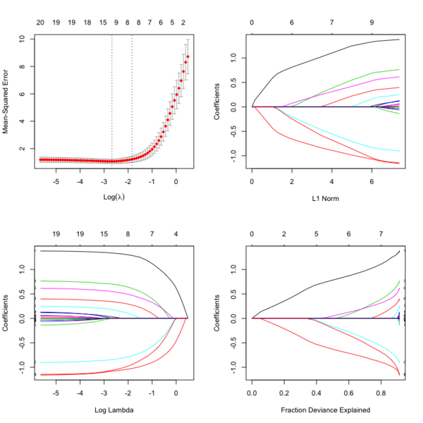
- Glmnet Vignette. It tries to minimize [math]\displaystyle{ RSS(\beta) + \lambda [(1-\alpha)\|\beta\|_2^2/2 + \alpha \|\beta\|_1] }[/math]. The elastic-net penalty is controlled by [math]\displaystyle{ \alpha }[/math], and bridge the gap between lasso ([math]\displaystyle{ \alpha = 1 }[/math]) and ridge ([math]\displaystyle{ \alpha = 0 }[/math]). Following is a CV curve (adaptive lasso) using the example from glmnet(). Two vertical lines are indicated: left one is lambda.min (that gives minimum mean cross-validated error) and right one is lambda.1se (the most regularized model such that error is within one standard error of the minimum). For the tuning parameter [math]\displaystyle{ \lambda }[/math],
- The larger the [math]\displaystyle{ \lambda }[/math], more coefficients are becoming zeros (think about coefficient path plots) and thus the simpler (more regularized) the model.
- If [math]\displaystyle{ \lambda }[/math] becomes zero, it reduces to the regular regression and if [math]\displaystyle{ \lambda }[/math] becomes infinity, the coefficients become zeros.
- In terms of the bias-variance tradeoff, the larger the [math]\displaystyle{ \lambda }[/math], the higher the bias and the lower the variance of the coefficient estimators.
File:Glmnetplot.svg File:Glmnet path.svg File:Glmnet l1norm.svg
set.seed(1010)
n=1000;p=100
nzc=trunc(p/10)
x=matrix(rnorm(n*p),n,p)
beta=rnorm(nzc)
fx= x[,seq(nzc)] %*% beta
eps=rnorm(n)*5
y=drop(fx+eps)
px=exp(fx)
px=px/(1+px)
ly=rbinom(n=length(px),prob=px,size=1)

## Full lasso
set.seed(999)
cv.full <- cv.glmnet(x, ly, family='binomial', alpha=1, parallel=TRUE)
plot(cv.full)  # cross-validation curve and two lambda's
plot(glmnet(x, ly, family='binomial', alpha=1), xvar="lambda", label=TRUE) # coefficient path plot
plot(glmnet(x, ly, family='binomial', alpha=1))  # L1 norm plot
log(cv.full$lambda.min) # -4.546394
log(cv.full$lambda.1se) # -3.61605
sum(coef(cv.full, s=cv.full$lambda.min) != 0) # 44

## Ridge Regression to create the Adaptive Weights Vector
set.seed(999)
cv.ridge <- cv.glmnet(x, ly, family='binomial', alpha=0, parallel=TRUE)
wt <- 1/abs(matrix(coef(cv.ridge, s=cv.ridge$lambda.min)
                   [, 1][2:(ncol(x)+1)] ))^1 ## Using gamma = 1, exclude intercept
## Adaptive Lasso using the 'penalty.factor' argument
set.seed(999)
cv.lasso <- cv.glmnet(x, ly, family='binomial', alpha=1, parallel=TRUE, penalty.factor=wt)
# defautl type.measure="deviance" for logistic regression
plot(cv.lasso)
log(cv.lasso$lambda.min) # -2.995375
log(cv.lasso$lambda.1se) # -0.7625655
sum(coef(cv.lasso, s=cv.lasso$lambda.min) != 0) # 34
- cv.glmnet() has a logical parameter parallel which is useful if a cluster or cores have been previously allocated
- Ridge regression and the LASSO
- Standard error/Confidence interval
- Standard Errors in GLMNET and Confidence intervals for Ridge regression
- Why SEs are not meaningful and are usually not provided in penalized regression?
- Hint: standard errors are not very meaningful for strongly biased estimates such as arise from penalized estimation methods.
- Penalized estimation is a procedure that reduces the variance of estimators by introducing substantial bias.
- The bias of each estimator is therefore a major component of its mean squared error, whereas its variance may contribute only a small part.
- Any bootstrap-based calculations can only give an assessment of the variance of the estimates.
- Reliable estimates of the bias are only available if reliable unbiased estimates are available, which is typically not the case in situations in which penalized estimates are used.
- Hottest glmnet questions from stackexchange.
- Standard errors for lasso prediction. There might not be a consensus on a statistically valid method of calculating standard errors for the lasso predictions.
- Code for Adaptive-Lasso for Cox's proportional hazards model by Zhang & Lu (2007). This can compute the SE of estimates. The weights are originally based on the maximizers of the log partial likelihood. However, the beta may not be estimable in cases such as high-dimensional gene data, or the beta may be unstable if strong collinearity exists among covariates. In such cases, robust estimators such as ridge regression estimators would be used to determine the weights.
- Some issues:
- With group of highly correlated features, Lasso tends to select amongst them arbitrarily.
- Often empirically ridge has better predictive performance than lasso but lasso leads to sparser solution
- Elastic-net (Zou & Hastie '05) aims to address these issues: hybrid between Lasso and ridge regression, uses L1 and L2 penalties.
- Gradient-Free Optimization for GLMNET Parameters
- Gsslasso Cox: a Bayesian hierarchical model for predicting survival and detecting associated genes by incorporating pathway information, Tang et al BMC Bioinformatics 2019
- Outlier detection and robust variable selection via the penalized weighted LAD-LASSO method Jiang 2020
- LASSO REGRESSION (HOME MADE)
- Course notes on Optimization for Machine Learning
Lambda
- A list of potential lambdas: see Linear Regression case. The λ sequence is determined by lambda.max and lambda.min.ratio.
- lambda.max is computed from the input x and y; it is the smallest value for lambda such that all the coefficients are zero.
- lambda.min.ratio (default is ifelse(nobs<nvars,0.01,0.0001)) is the ratio of smallest value of the generated λ sequence (say lambda.min) to lambda.max.
- The program then generated nlambda values linear on the log scale from lambda.max down to lambda.min.
- Choosing hyper-parameters (α and λ) in penalized regression by Florian Privé
- lambda.min vs lambda.1se
- The lambda.1se represents the value of λ in the search that was simpler than the best model (lambda.min), but which has error within 1 standard error of the best model ( lambda.min < lambda.1se ). In other words, using the value of lambda.1se as the selected value for λ results in a model that is slightly simpler than the best model but which cannot be distinguished from the best model in terms of error given the uncertainty in the k-fold CV estimate of the error of the best model.
- The lambda.min option refers to value of λ at the lowest CV error. The error at this value of λ is the average of the errors over the k folds and hence this estimate of the error is uncertain.
- https://www.rdocumentation.org/packages/glmnet/versions/2.0-10/topics/glmnet
- glmnetUtils: quality of life enhancements for elastic net regression with glmnet
- Mixing parameter: alpha=1 is the lasso penalty, and alpha=0 the ridge penalty and anything between 0–1 is Elastic net.
- RIdge regression uses Euclidean distance/L2-norm as the penalty. It won't remove any variables.
- Lasso uses L1-norm as the penalty. Some of the coefficients may be shrunk exactly to zero.
- In ridge regression and lasso, what is lambda?
- Lambda is a penalty coefficient. Large lambda will shrink the coefficients.
- cv.glment()$lambda.1se gives the most regularized model such that error is within one standard error of the minimum
- A deep dive into glmnet: penalty.factor, standardize, offset
- Lambda sequence is not affected by the "penalty.factor"
- How "penalty.factor" used by the objective function may need to be corrected
- A deep dive into glmnet: predict.glmnet
Underfittig, overfitting and relaxed lasso
- https://cran.r-project.org/web/packages/glmnet/vignettes/relax.pdf
- The Relaxed Lasso: A Better Way to Fit Linear and Logistic Models
- Overfitting: small lambda, lots of non-zero coefficients
- Underfitting: large lambda, not enough variables
- Relaxed Lasso by Nicolai Meinshausen
- Why is “relaxed lasso” different from standard lasso?
- https://web.stanford.edu/~hastie/TALKS/hastieJSM2017.pdf#page=13
- Stabilizing the lasso against cross-validation variability
Plots
library(glmnet)
data(QuickStartExample)

cvfit = cv.glmnet(x, y)
fit = glmnet(x, y)

oldpar <- par(mfrow=c(2,2))
plot(cvfit) # mse vs log(lambda)
plot(fit) # coef vs L1 norm
plot(fit, xvar = "lambda", label = TRUE) # coef vs log(lambda)
plot(fit, xvar = "dev", label = TRUE) # coef vs Fraction Deviance Explained
par(oldpar)
Relaxed fit and [math]\displaystyle{ \gamma }[/math] parameter
https://cran.r-project.org/web/packages/glmnet/vignettes/relax.pdf
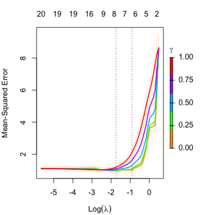
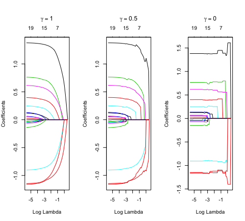
Relaxed fit: Take a glmnet fitted object, and then for each lambda, refit the variables in the active set without any penalization.
Suppose the glmnet fitted linear predictor at [math]\displaystyle{ \lambda }[/math] is [math]\displaystyle{ \hat\eta_\lambda(x) }[/math] and the relaxed version is [math]\displaystyle{ \tilde\eta_\lambda(x) }[/math]. We also allow for shrinkage between the two:
- [math]\displaystyle{ \begin{align} \tilde \eta_{\lambda,\gamma}= \gamma\hat\eta_\lambda(x) + (1-\gamma)\tilde\eta_\lambda(x). \end{align} }[/math]
[math]\displaystyle{ \gamma\in[0,1] }[/math] is an additional tuning parameter which can be selected by cross validation.
The debiasing will potentially improve prediction performance, and CV will typically select a model with a smaller number of variables.
library(glmnet) data(QuickStartExample) fitr=glmnet(x,y, relax=TRUE) set.seed(1) cfitr=cv.glmnet(x,y,relax=TRUE) c(fitr$lambda.min, fitr$lambda.1se) # [1] 0.08307327 0.15932708 plot(cfitr),oldpar <- par(mfrow=c(1,3), mar = c(5,4,6,2)) plot(fitr, main = expression(gamma == 1)) plot(fitr,gamma=0.5, main = expression(gamma == .5)) plot(fitr,gamma=0, main = expression(gamma == 0)) par(oldpar) |
Special cases:
set.seed(1) fitr2=cv.glmnet(x,y,gamma=0,relax=TRUE) # default gamma = c(0, 0.25, 0.5, 0.75, 1) plot(fitr2) c(fitr2$lambda.min, fitr2$lambda.1se) # [1] 0.08307327 0.15932708 |
Adaptive lasso
Oracle property and adaptive lasso
- Variable Selection via Nonconcave Penalized Likelihood and Its Oracle Properties, Fan & Li (2001) JASA
- Adaptive Lasso: What it is and how to implement in R. Adaptive lasso weeks to minimize [math]\displaystyle{ RSS(\beta) + \lambda \sum_1^p \hat{\omega}_j |\beta_j| }[/math] where [math]\displaystyle{ \lambda }[/math] is the tuning parameter, [math]\displaystyle{ \hat{\omega}_j = \frac{1}{(|\hat{\beta}_j^{ini}|)^\gamma} }[/math] is the adaptive weights vector and [math]\displaystyle{ \hat{\beta}_j^{ini} }[/math] is an initial estimate of the coefficients obtained through ridge regression. Adaptive Lasso ends up penalizing more those coefficients with lower initial estimates. [math]\displaystyle{ \gamma }[/math] is a positive constant for adjustment of the adaptive weight vector, and the authors suggest the possible values of 0.5, 1 and 2.
- When n goes to infinity, [math]\displaystyle{ \hat{\omega}_j |\beta_j| }[/math] converges to [math]\displaystyle{ I(\beta_j \neq 0) }[/math]. So the adaptive Lasso procedure can be regarded as an automatic implementation of best-subset selection in some asymptotic sense.
- What is the oracle property of an estimator? An oracle estimator must be consistent in 1) variable selection and 2) consistent parameter estimation.
- (Linear regression) The adaptive lasso and its oracle properties Zou (2006, JASA)
- (Cox model) Adaptive-LASSO for Cox's proportional hazard model by Zhang and Lu (2007, Biometrika)
- When the LASSO fails???. Adaptive lasso is used to demonstrate its usefulness.
Cyclic coordinate descent
A deep dive into glmnet: type.gaussian
Survival data
- The sum of errors term can be replaced with [math]\displaystyle{ -l(\beta, \gamma) }[/math], where [math]\displaystyle{ l(\cdot, \cdot) }[/math] stands for the log-likelihood function and [math]\displaystyle{ \gamma }[/math] for the intercept. See The lasso method for variable selection in the cox model 1997.
- Cox regression: Estimation by Patrick Breheny
Prediction
- Comparison of pathway and gene-level models for cancer prognosis prediction Zheng, 2020
- CAncer bioMarker Prediction Pipeline (CAMPP)—A standardized framework for the analysis of quantitative biological data Terkelsen, 2020
LASSO vs Least angle regression
- https://web.stanford.edu/~hastie/Papers/LARS/LeastAngle_2002.pdf
- Least Angle Regression, Forward Stagewise and the Lasso
- https://www.quora.com/What-is-Least-Angle-Regression-and-when-should-it-be-used
- A simple explanation of the Lasso and Least Angle Regression
- https://stats.stackexchange.com/questions/4663/least-angle-regression-vs-lasso
- https://cran.r-project.org/web/packages/lars/index.html
Tidymodel
Lasso regression using tidymodels and #tidytuesday data for the office
Binary particle swarm optimization (BPSO)
An efficient gene selection method for microarray data based on LASSO and BPSO


