Longitudinal
Mixed Effect Model
- Paper by Laird and Ware 1982
- Random effects vs fixed effects model: There may be factors related to country/region (random variable) which may result in different patients’ responses to the vaccine, and, not all countries are included in the study.
- John Fox's Linear Mixed Models Appendix to An R and S-PLUS Companion to Applied Regression. Very clear. It provides 2 typical examples (hierarchical data and longitudinal data) of using the mixed effects model. It also uses Trellis plots to examine the data.
- Chapter 10 Random and Mixed Effects from Modern Applied Statistics with S by Venables and Ripley.
- (Book) lme4: Mixed-effects modeling with R by Douglas Bates.
- (Book) Mixed-effects modeling in S and S-Plus by José Pinheiro and Douglas Bates.
- Simulation and power analysis of generalized linear mixed models
- Linear mixed-effect models in R by poissonisfish
- Dealing with correlation in designed field experiments: part II
- Mixed Models in R by Michael Clark
- Mixed models in R: a primer
- Chapter 4 Simulating Mixed Effects by Lisa DeBruine
- Linear mixed effects models (video) by Clapham. Output for y ~ x + (x|group) model.
y ~ x + (1|group)  # random intercepts, same slope for groups

y ~ x + (x|group)  # random intercepts & slopes for groups

y ~ color + (color|green/gray) # nested random effects

y ~ color + (color|green) + (color|gray) # crossed random effects
- linear mixed effects models in R lme4
- Using Random Effects in Models by rcompanion
library(nlme)
lme(y ~ 1 + randonm = ~1 | Random) # one-way random model

lme(y ~ Fix + random = ~1 | Random) # two-way mixed effect model

# https://stackoverflow.com/a/36415354
library(lme4)
fit <- lmer(mins ~ Fix1 + Fix2 + (1|Random1) + (1|Random2) +
                (1|Year/Month), REML=FALSE)
- Random effects and penalized splines are the same thing
- Introduction to linear mixed models
- Fitting 'complex' mixed models with 'nlme'
- A random variable has to consist of at least 5 levels. An Introduction to Linear Mixed Effects Models (video)
- A Guide on Data Analysis Mike Nguyen
Repeated measure
-
R Tutorial: Linear mixed-effects models part 1- Repeated measures ANOVA
words ~ drink + (1|subj) # random intercepts
Trajectories
- In longitudinal data analysis, trajectories refer to the patterns of change over time in a variable or set of variables for an individual or group of individuals1. These patterns can be used to identify typical trajectories in longitudinal data using mixed effects models1. The result is summarized in terms of an average trajectory plus measures of the individual variations around this average
- Identifying typical trajectories in longitudinal data: modelling strategies and interpretations 2020
- Visualise longitudinal data
- An example: a model that there are random intercepts and slopes for each subject:
[math]\displaystyle{ y_{ij} = \beta_0 + \beta_1 x_{ij} + b_{0i} + b_{1i} x_{ij} + e_{ij}
}[/math]
- [math]\displaystyle{ y_{ij} }[/math] is the reaction time for subject i at time j
- [math]\displaystyle{ \beta_0, \beta_1 }[/math] are fixed intercept and slope
- [math]\displaystyle{ x_{ij} }[/math] is the number of days since the start of the study for subject i at time j
- [math]\displaystyle{ b_{0i}, b_{1i} }[/math] are the random intercept & slope for subject i
- [math]\displaystyle{ e_{ij} }[/math] is the residual error for subject i at time j
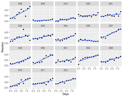
> library(lme4) > data(sleepstudy) # from lme4 > # Fit a mixed effects model with random intercepts and slopes for each subject > model <- lmer(Reaction ~ Days + (Days | Subject), sleepstudy) > > # Plot the fitted model > plot(model, type = "l") > summary(model) Linear mixed model fit by REML ['lmerMod'] Formula: Reaction ~ Days + (Days | Subject) Data: sleepstudy REML criterion at convergence: 1743.6 Scaled residuals: Min 1Q Median 3Q Max -3.9536 -0.4634 0.0231 0.4634 5.1793 Random effects: Groups Name Variance Std.Dev. Corr Subject (Intercept) 612.10 24.741 Days 35.07 5.922 0.07 Residual 654.94 25.592 Number of obs: 180, groups: Subject, 18 Fixed effects: Estimate Std. Error t value (Intercept) 251.405 6.825 36.838 Days 10.467 1.546 6.771 Correlation of Fixed Effects: (Intr) Days -0.138- The fixed effect estimate for Days is 10.4673, which means that on average, reaction times decrease by 10.4673 milliseconds per day.
- The random intercept variance is 612.09, which means that there is considerable variation in the baseline reaction times between subjects.
- The random slope variance is 35.07, which means that there is considerable variation in the rate of change of reaction times over time between subjects.
- It seems no p-values are returned. See Three ways to get parameter-specific p-values from lmer & How to obtain the p-value (check significance) of an effect in a lme4 mixed model?
- To exclude the random slope term, we can use (1 | Subject)
- To exclude the random intercept term, we can use (0 + Days | Subject)
- To exclude the fix intercept term, we can use y ~ -1 + x + (Days | Subject)
library(nlme) model2 <- lme(Reaction ~ Days, random = ~ Days | Subject, data = sleepstudy) > summary(model2) Linear mixed-effects model fit by REML Data: sleepstudy AIC BIC logLik 1755.628 1774.719 -871.8141 Random effects: Formula: ~Days | Subject Structure: General positive-definite, Log-Cholesky parametrization StdDev Corr (Intercept) 24.740241 (Intr) Days 5.922103 0.066 Residual 25.591843 Fixed effects: Reaction ~ Days Value Std.Error DF t-value (Intercept) 251.40510 6.824516 161 36.83853 Days 10.46729 1.545783 161 6.77151 p-value (Intercept) 0 Days 0 Correlation: (Intr) Days -0.138 Standardized Within-Group Residuals: Min Q1 Med Q3 -3.95355735 -0.46339976 0.02311783 0.46339621 Max 5.17925089 Number of Observations: 180 Number of Groups: 18- To exclude the random slope term, we can use random = ~1 | Subject.
- To exclude the random intercept, we can use random = ~Days - 1 | Subject.
Graphical display using facet_wrap().
- lmerTest - Tests in Linear Mixed Effects Models.
The ranova() function in the lmerTest package is used to compute an ANOVA-like table with tests of random-effect terms in a mixed-effects model. Paper in JSS 2017.
# Fixed effect
> anova(model)
Type III Analysis of Variance Table with Satterthwaite's method
     Sum Sq Mean Sq NumDF DenDF F value    Pr(>F)
Days  30031   30031     1    17  45.853 3.264e-06 ***
---
Signif. codes:
0 ‘***’ 0.001 ‘**’ 0.01 ‘*’ 0.05 ‘.’ 0.1 ‘ ’ 1

> anova(model2)
            numDF denDF   F-value p-value
(Intercept)     1   161 1454.0766  <.0001
Days            1   161   45.8534  <.0001

# Random effect
> ranova(model)
ANOVA-like table for random-effects: Single term deletions

Model:
Reaction ~ Days + (Days | Subject)
                         npar  logLik    AIC    LRT Df
<none>                      6 -871.81 1755.6
Days in (Days | Subject)    4 -893.23 1794.5 42.837  2
                         Pr(>Chisq)
<none>
Days in (Days | Subject)   4.99e-10 ***
---
Signif. codes:
0 ‘***’ 0.001 ‘**’ 0.01 ‘*’ 0.05 ‘.’ 0.1 ‘ ’ 1

variancePartition
variancePartition Quantify and interpret divers of variation in multilevel gene expression experiments
GEE/generalized estimating equations
- https://en.wikipedia.org/wiki/Generalized_estimating_equation
- Literatures:
- Longitudinal Data Analysis for Discrete and Continuous Outcomes Scott L. Zeger and Kung-Yee Liang Biometrics 1986
- Longitudinal data analysis using generalized linear models. Liang, K., and S. L. Zeger (1986) Biometrika.
- Analysis of Longitudinal Data (Oxford Statistical Science Series) 2nd edition by Peter Diggle, Patrick Heagerty, Kung-Yee Liang, and Scott Zeger
- Youtube
- 12.1 - Introduction to Generalized Estimating Equations from PennState
- 12.2 - Modeling Binary Clustered Responses which shows the "exchangeable" correlation structure
- gee package. First version 1999.
- geepack package. First version 2002.
- Getting Started with Generalized Estimating Equations.
- The Working correlation matrix output from the gee() function when "exchangeable" correlation was used. The dimension of "working correlation" is the number of observations per subject/id. Question: why the diagonal elements of the working correlation is sometimes 0 instead of 1 in my data.
- The Estimated Scale Parameter is the dispersion parameter.
- Chapter 15 GEE, Binary Outcome: Respiratory Illness from Encyclopedia of Quantitative Methods in R, vol. 5: Multilevel Models.
- SAS/STAT 14.1 User’s Guide The GEE Procedure
- Fast Pure R Implementation of GEE: Application of the Matrix Package
- One example
library(geepack)

# load data
data("cbpp", package = "lme4")
cbpp[1:3, ]
#   herd incidence size period
# 1    1         2   14      1
# 2    1         3   12      2
# 3    1         4    9      3
with(cbpp, table(herd, period))
    period
herd 1 2 3 4
  1  1 1 1 1
  2  1 1 1 0
  3  1 1 1 1
  4  1 1 1 1
  5  1 1 1 1
  6  1 1 1 1
  7  1 1 1 1
  8  1 0 0 0
  9  1 1 1 1
  10 1 1 1 1
  11 1 1 1 1
  12 1 1 1 1
  13 1 1 1 1
  14 1 1 1 1
  15 1 1 1 1

# fit GEE model with logit link
fit <- geeglm(cbind(incidence, size - incidence) ~ period, id = herd,
              family = binomial("logit"), corstr = "exchangeable", data = cbpp)

# summary of the model
summary(fit)
 Coefficients:
            Estimate Std.err  Wald Pr(>|W|)
(Intercept)   -1.270   0.276 21.24  4.0e-06 ***
period2       -1.156   0.436  7.04   0.0080 **
period3       -1.284   0.491  6.84   0.0089 **
period4       -1.754   0.375 21.85  2.9e-06 ***
---
Signif. codes:
0 ‘***’ 0.001 ‘**’ 0.01 ‘*’ 0.05 ‘.’ 0.1 ‘ ’ 1

Correlation structure = exchangeable
Estimated Scale Parameters:

            Estimate Std.err
(Intercept)    0.134  0.0542
  Link = identity

Estimated Correlation Parameters:
      Estimate Std.err
alpha   0.0414   0.129
Number of clusters:   15  Maximum cluster size: 4

summary(fit)$coefficients
            Estimate Std.err  Wald Pr(>|W|)
(Intercept)    -1.27   0.276 21.24 4.04e-06
period2        -1.16   0.436  7.04 7.99e-03
period3        -1.28   0.491  6.84 8.90e-03
period4        -1.75   0.375 21.85 2.94e-06

# extract robust variance-covariance matrix
vcov_fit <- vcovHC(fit, type = "HC")

# compute confidence intervals for coefficients
library(sandwich)

vcov_fit <- vcovHC(fit, type = "HC")
ci <- coef(fit) + cbind(qnorm(0.025), qnorm(0.975)) * sqrt(diag(vcov_fit))
colnames(ci) <- c("2.5 %", "97.5 %")
print(ci)
[math]\displaystyle{ \operatorname{logit}\left(\frac{p_{ij}}{1 - p_{ij}}\right) = \beta_0 + \beta_1 \cdot \text{period}_{ij} + u_j }[/math] where [math]\displaystyle{ p_{ij} }[/math] is the probability of a positive outcome (i.e., an incidence) for
- the [math]\displaystyle{ i }[/math]-th animal/observation in herd(group/subject) [math]\displaystyle{ j }[/math], and
- [math]\displaystyle{ \text{period}_{ij} }[/math] is a categorical predictor variable indicating the period of observation for herd/subject [math]\displaystyle{ j }[/math] and observation [math]\displaystyle{ i }[/math].
- The parameters [math]\displaystyle{ \beta_0 }[/math] and [math]\displaystyle{ \beta_1 }[/math] represent the intercept and the effect of the period variable, respectively.
- The [math]\displaystyle{ u_j }[/math] is the random subject-specific effect. The random effects [math]\displaystyle{ u_j }[/math] are assumed to follow a multivariate normal distribution with mean 0 and covariance matrix [math]\displaystyle{ \Sigma }[/math].
- The correlation structure of the random effects is specified as "exchangeable", which means that any two random effects from the same subject have the same correlation.
Compare models
- 015. GEE in Practice: Example on COVID-19 Test Positivity Data. QIC is available in the geepack package.
- geeglm was used.
- simple scatterplot by plot() with y=positivity_rate, x=time
- lattice::xyplot()
xyplot(positivity_rate ~ time|ID,
       groups = ID,
       subset = ID %in% sampled_idx,
       data= covid,
       panel = function(x, y) {
         panel.xyplot(x, y, plot='p')
         panel.linejoin(x, y,
                       fun=mean,
                       horizontal = F,
                       lwd=2, col=1)
       })
- create a factor
covid$size_factor <-  cut(covid$estimat_pop,
                   breaks = quantile(unique(covid$estimated_pop)),
                   include.lowest = TRUE,
                   lables = FALSE)  |>  as.factor()

xyplot(positivity_rate ~ time|size_factor, # size_factor is like a facet
       groups = ID,
       data= covid,
       panel = function(x, y) {
         panel.xyplot(x, y, plot='p')
         panel.linejoin(x, y,
                       fun=mean,
                       horizontal = F,
                       lwd=2, col=1)
       })
- Residual vs predict plot from plot(fit) can be used to evaluate which correlation structure is better.
- QIC() output and what metric can be used for [model selection. QIC & CIC are most useful for selecting correlation structure. QICU is most useful for comparing models with the same correlation structure but different mean structure.
- Analysis of panel data in R using Generalized Estimating Equations which uses the MESS package
Simulation
- How to simulate data for generalized estimating equations (GEE) with logistic link function?
- We generate some example data with repeated measurements. In this simulated data, we have 100 subjects, each measured at 5 time points.
# Load the geepack package
library(geepack)

# Generate some example data with repeated measurements
set.seed(123)
n <- 100  # Number of subjects
time <- rep(1:5, each = n)  # Time points
subject <- rep(1:n, times = 5)  # Subject IDs
y <- rnorm(n * 5, mean = time * 0.5 + subject * 0.2)  # Simulated response variable

# Create a data frame
data <- data.frame(subject, time, y)

# Fit a GEE model using geeglm
# In this example, we assume an exchangeable correlation structure
model <- geeglm(y ~ time, id = subject, data = data, family = gaussian, corstr = "exchangeable")

# Summary of the GEE model
summary(model)
# Coefficients:
#             Estimate Std.err   Wald Pr(>|W|)
# (Intercept)  10.1039  0.6222 263.69  < 2e-16 ***
# time          0.5102  0.1877   7.39  0.00656 **
# ---
# Signif. codes:  0 ‘***’ 0.001 ‘**’ 0.01 ‘*’ 0.05 ‘.’ 0.1 ‘ ’ 1
#
# Correlation structure = exchangeable
# Estimated Scale Parameters:
#
#            Estimate Std.err
# (Intercept)    35.09   1.444
#   Link = identity
#
# Estimated Correlation Parameters:
#       Estimate Std.err
# alpha        0       0
# Number of clusters:   500  Maximum cluster size: 1

model2 = geeglm(y ~ time, id = subject, data = data, family = gaussian, corstr = "ind")
summary(model2)
#  Coefficients:
#             Estimate Std.err   Wald Pr(>|W|)
# (Intercept)   10.104   0.622 263.68   <2e-16 ***
# time           0.510   0.188   7.39   0.0066 **
# ---
# Signif. codes:  0 ‘***’ 0.001 ‘**’ 0.01 ‘*’ 0.05 ‘.’ 0.1 ‘ ’ 1
#
# Correlation structure = independence
# Estimated Scale Parameters:
#
#             Estimate Std.err
# (Intercept)     35.1    1.44
# Number of clusters:   500  Maximum cluster size: 1
gee vs geepack packages
GENERALIZED ESTIMATING EQUATIONS (GEE) by Practical Statistics (Rebecca Barter).
Subject-specific versus Population-averaged.
GEE estimates population-averaged model parameters and their standard errors.
library("geepack")
data(dietox)
dietox$Cu <- as.factor(dietox$Cu)
dietox$Evit <- as.factor(dietox$Evit)
mf <- formula(Weight ~ Time + Evit + Cu)

geeEx <- geeglm(mf, id=Pig, data=dietox, family=gaussian, corstr="ex")
summary(geeEx)

Call:
geeglm(formula = mf, family = gaussian, data = dietox, id = Pig,
    corstr = "ex")

 Coefficients:
            Estimate Std.err    Wald Pr(>|W|)
(Intercept)  15.0984  1.4206  112.96   <2e-16 ***
Time          6.9426  0.0796 7605.79   <2e-16 ***
EvitEvit100   2.0414  1.8431    1.23     0.27
EvitEvit200  -1.1103  1.8452    0.36     0.55
CuCu035      -0.7652  1.5354    0.25     0.62
CuCu175       1.7871  1.8189    0.97     0.33
---
Signif. codes:  0 ‘***’ 0.001 ‘**’ 0.01 ‘*’ 0.05 ‘.’ 0.1 ‘ ’ 1

Correlation structure = exchangeable
Estimated Scale Parameters:

            Estimate Std.err
(Intercept)     48.3    9.31
  Link = identity

Estimated Correlation Parameters:
      Estimate Std.err
alpha    0.766  0.0326
Number of clusters:   72  Maximum cluster size: 12
Note that the correlation estimate obtained from geeglm() is 0.766 = summary(geeEx)$geese$correlation$estimate.
gee() can show the complete correlation structure in the output. The correlation estimate is 0.761 =summary(geeEx2)$working.correlation[1, 2].
geeEx2 = gee::gee(Weight ~ Time + Evit + Cu, id=Pig, data=dietox, family=gaussian, corstr="exchangeable")
summary(geeEx2)
Beginning Cgee S-function, @(#) geeformula.q 4.13 98/01/27
running glm to get initial regression estimate
(Intercept)        Time EvitEvit100 EvitEvit200     CuCu035     CuCu175
     15.073       6.948       2.081      -1.113      -0.789       1.777

 GEE:  GENERALIZED LINEAR MODELS FOR DEPENDENT DATA
 gee S-function, version 4.13 modified 98/01/27 (1998)

Model:
 Link:                      Identity
 Variance to Mean Relation: Gaussian
 Correlation Structure:     Exchangeable

Call:
gee::gee(formula = Weight ~ Time + Evit + Cu, id = Pig, data = dietox,
    family = gaussian, corstr = "exchangeable")

Summary of Residuals:
    Min      1Q  Median      3Q     Max
-34.396  -3.245   0.903   4.127  20.157


Coefficients:
            Estimate Naive S.E. Naive z Robust S.E. Robust z
(Intercept)   15.098     1.6955   8.905      1.4206   10.628
Time           6.943     0.0337 205.820      0.0796   87.211
EvitEvit100    2.041     1.7991   1.135      1.8431    1.108
EvitEvit200   -1.110     1.7813  -0.623      1.8452   -0.602
CuCu035       -0.765     1.7813  -0.430      1.5354   -0.498
CuCu175        1.787     1.7991   0.993      1.8189    0.982

Estimated Scale Parameter:  48.6
Number of Iterations:  2

Working Correlation
       [,1]  [,2]  [,3]  [,4]  [,5]  [,6]  [,7]  [,8]  [,9] [,10] [,11] [,12]
 [1,] 1.000 0.761 0.761 0.761 0.761 0.761 0.761 0.761 0.761 0.761 0.761 0.761
 [2,] 0.761 1.000 0.761 0.761 0.761 0.761 0.761 0.761 0.761 0.761 0.761 0.761
 [3,] 0.761 0.761 1.000 0.761 0.761 0.761 0.761 0.761 0.761 0.761 0.761 0.761
 [4,] 0.761 0.761 0.761 1.000 0.761 0.761 0.761 0.761 0.761 0.761 0.761 0.761
 [5,] 0.761 0.761 0.761 0.761 1.000 0.761 0.761 0.761 0.761 0.761 0.761 0.761
 [6,] 0.761 0.761 0.761 0.761 0.761 1.000 0.761 0.761 0.761 0.761 0.761 0.761
 [7,] 0.761 0.761 0.761 0.761 0.761 0.761 1.000 0.761 0.761 0.761 0.761 0.761
 [8,] 0.761 0.761 0.761 0.761 0.761 0.761 0.761 1.000 0.761 0.761 0.761 0.761
 [9,] 0.761 0.761 0.761 0.761 0.761 0.761 0.761 0.761 1.000 0.761 0.761 0.761
[10,] 0.761 0.761 0.761 0.761 0.761 0.761 0.761 0.761 0.761 1.000 0.761 0.761
[11,] 0.761 0.761 0.761 0.761 0.761 0.761 0.761 0.761 0.761 0.761 1.000 0.761
[12,] 0.761 0.761 0.761 0.761 0.761 0.761 0.761 0.761 0.761 0.761 0.761 1.000
GEE vs. mixed effects models
- https://stats.stackexchange.com/a/16415
- Getting Started with Generalized Estimating Equations
- It uses "gee", "lme4", "geepack" packages for model fittings
dep_gee2 <- gee(depression ~ diagnose + drug*time, data = dat, id = id, family = binomial, corstr = "exchangeable")- How does the GEE model with the exchangeable correlation structure compare to a Generalized Mixed-Effect model. We allow the intercept to be conditional on subject. This means we’ll get 340 subject_specific models with different intercepts but identical coefficients for everything else. The model coefficients listed under “Fixed effects” are almost identical to the GEE coefficients. ?glmer for GLMMs/Generalized Linear Mixed-Effects Models.
library(lme4) # version 1.1-31
dep_glmer <- glmer(depression ~ diagnose + drug*time + (1|id),
               data = dat, family = binomial)
summary(dep_glmer, corr = FALSE)
dep_gee4 <- geeglm(depression ~ diagnose + drug*time, data = dat, id = id, family = binomial, corstr = "exchangeable")
- "ggeffects" package for plotting. The emmeans function calculates marginal effects and works for both GEE and mixed-effect models.
library(ggeffects)
library(emmeans)
plot(ggemmeans(dep_glmer, terms = c("time", "drug"),
               condition = c(diagnose = "severe"))) +
  ggplot2::ggtitle("GLMER Effect plot")

data.frame(ggemmeans(dep_glmer, terms = c("time", "drug"),
           condition = c(diagnose = "severe")) )
  x predicted std.error conf.low conf.high    group
1 0     0.207     0.175    0.156     0.269 standard
2 0     0.197     0.187    0.146     0.262      new
3 1     0.297     0.119    0.251     0.348 standard
4 1     0.525     0.126    0.463     0.586      new
5 2     0.407     0.156    0.335     0.482 standard
6 2     0.832     0.217    0.764     0.883      new
filter(dat, diagnose == "severe") %>%
   group_by(drug, time) %>%
   summarize(mean = mean(depression))
  drug      time  mean
  <fct>    <int> <dbl>
1 standard     0 0.21
2 standard     1 0.28
3 standard     2 0.46
4 new          0 0.178
5 new          1 0.5
6 new          2 0.833

plot(ggemmeans(dep_gee4, terms = c("time", "drug"),
               condition = c(diagnose = "severe"))) +
  ggplot2::ggtitle("GEE Effect plot")
- While both methods are used for modeling correlated data, there are some key differences between them.
- Assumptions: The key difference between GEE and nlme is that GEE makes fewer assumptions about the underlying data structure. GEE assumes that the mean structure is correctly specified, but the correlation structure is unspecified. In contrast, nlme assumes that both the mean and the variance-covariance structure are correctly specified.
- Model flexibility: GEE is a more flexible model than nlme because it allows for modeling the mean and variance of the response separately. This means that GEE is more suitable for modeling data with non-normal errors, such as count or binary data. In contrast, nlme assumes that the errors are normally distributed and allows for modeling the mean and variance jointly.
- Inference: Another key difference between GEE and nlme is the type of inference they provide. GEE provides marginal inference, which means that it estimates the population-averaged effect of the predictor variables on the response variable. In contrast, nlme provides conditional inference, which means that it estimates the subject-specific effect of the predictor variables on the response variable.
- Computation: The computation involved in fitting GEE and nlme models is also different. GEE uses an iterative algorithm to estimate the model parameters, while nlme uses a maximum likelihood estimation approach. The computational complexity of GEE is lower than that of nlme, making it more suitable for large datasets.
- In summary, GEE and nlme are two popular models used for analyzing longitudinal data. The main differences between the two models are the assumptions they make, model flexibility, inference type, and computational complexity. GEE is a more flexible model that makes fewer assumptions and provides marginal inference, while nlme assumes normality of errors and provides conditional inference.
Independent correlation
If you assume an independent correlation structure in a Generalized Estimating Equation (GEE) model, the GEE estimates are the same as those obtained from a Generalized Linear Model (GLM) or Ordinary Least Squares (OLS) if the dependent variable is normally distributed and no correlation within responses are assumed².
However, the standard errors in a GEE model will be different from those in a GLM or OLS model. This is because GEE takes into account the within-subject correlation, which can lead to more efficient estimates¹. If this correlation is not taken into account, the regression estimates would be less efficient, meaning they would be more widely scattered around the true population value¹.
It's important to note that while the point estimates might be the same, the interpretation of these estimates differs between GEE and GLM/OLS models. In a GEE model, you're making inferences about the population average response, whereas in a GLM/OLS model, you're making inferences about individual-level effects¹.
References:
- GEE: choosing proper working correlation structure.
- GEE for Repeated Measures Analysis | Columbia Public Health.