Longitudinal
Longitudinal Data Analysis
- Longitudinal Data Analysis by Patrick Heagerty
- Core Guide: Longitudinal Data Analysis by Duke Global Health
- Chapter 4 Models for Longitudinal Data lme4
- **A review of Longitudinal Data Analysis in R. Very nice!
- Chapter 6: Multilevel Modeling R for Researchers. GEE & Mixed Effects.
- Longitudinal Data Analysis for the Behavioral Sciences Using R by Jeffrey Long.
- Methods and Applications of Longitudinal Data Analysis Xian Liu
Mixed Effect Model
- Paper by Laird and Ware 1982
- Random effects vs fixed effects model: There may be factors related to country/region (random variable) which may result in different patients’ responses to the vaccine, and, not all countries are included in the study.
- John Fox's Linear Mixed Models Appendix to An R and S-PLUS Companion to Applied Regression. Very clear. It provides 2 typical examples (hierarchical data and longitudinal data) of using the mixed effects model. It also uses Trellis plots to examine the data.
- Chapter 10 Random and Mixed Effects from Modern Applied Statistics with S by Venables and Ripley.
- (Book) lme4: Mixed-effects modeling with R by Douglas Bates.
- (Book) Mixed-effects modeling in S and S-Plus by José Pinheiro and Douglas Bates.
- Simulation and power analysis of generalized linear mixed models
- Linear mixed-effect models in R by poissonisfish
- Dealing with correlation in designed field experiments: part II
- Mixed Models in R by Michael Clark
- Mixed models in R: a primer
- Chapter 4 Simulating Mixed Effects by Lisa DeBruine
- Linear mixed effects models (video) by Clapham. Output for y ~ x + (x|group) model.
y ~ x + (1|group)  # random intercepts, same slope for groups

y ~ x + (x|group)  # random intercepts & slopes for groups

y ~ color + (color|green/gray) # nested random effects

y ~ color + (color|green) + (color|gray) # crossed random effects
- linear mixed effects models in R lme4
- Using Random Effects in Models by rcompanion
library(nlme)
lme(y ~ 1 + randonm = ~1 | Random) # one-way random model

lme(y ~ Fix + random = ~1 | Random) # two-way mixed effect model

# https://stackoverflow.com/a/36415354
library(lme4)
fit <- lmer(mins ~ Fix1 + Fix2 + (1|Random1) + (1|Random2) +
                (1|Year/Month), REML=FALSE)
- Random effects and penalized splines are the same thing
- Introduction to linear mixed models
- Fitting 'complex' mixed models with 'nlme'
- A random variable has to consist of at least 5 levels. An Introduction to Linear Mixed Effects Models (video)
- A Guide on Data Analysis Mike Nguyen
- FAQs on mixed-effects models, Mixed-effects models in R, and a new tool for data simulation by Pablo Bernabeu.
Repeated measure: aov()
- Repeated Measures ANOVA in R
- One Way repeated measure ANOVA in R.
- Data contains subject (random effect), time (fixed effect) and response.
- The model in the following code tests whether there are significant differences in the response across time while considering within-subject variability.
- Since we simulated increasing means (51, 54, 59), we expect a statistically significant effect of time.
- A one-way ANOVA tests only if at least one time point is different, not the direction of change. So. if we simulate means (51, 59, 54) with a large number of subjects and small random noise, the ANOVA may still return a significant p-value. However, if the variance in individual responses overlaps significantly across time points, it might fail to reach statistical significance.
- The simulated code does not include between-subject variability - each subject's responses are generated from the same population mean at each time point without individual subject-level shifts.
- The Error structure Error(subject/time) splits the variance into:
- subject: Captures variability between subjects.
- subject:time: Captures within-subject (time) effects.
- The math model is [math]\displaystyle{ y_{it} = \mu + \alpha_t + \epsilon_{it}, }[/math] where [math]\displaystyle{ \epsilon_{it} }[/math] is the residual error for subject i at time t, capturing the within-subject variability at time t.
set.seed(123)

# Define parameters
num_subjects <- 10  # Number of subjects
num_timepoints <- 3  # Number of time points

# Create a data frame
subject <- factor(rep(1:num_subjects, each = num_timepoints))
time <- factor(rep(1:num_timepoints, times = num_subjects))

# Assume baseline mean of 50 with small changes over time and some subject variability
# sd controls within-subject variability
response <- rnorm(num_subjects * num_timepoints, mean = 50 + as.numeric(time) * 2, sd = 2)

data <- data.frame(subject, time, response)

# Fit one-way repeated measures ANOVA model.
# subject/time means time is nested within subject
# It accounts for within-subject variation.
# It only tests the time effect.
model <- aov(response ~ time + Error(subject/time), data = data)

# The first block shows no test because subjects are considered random.
# The second Error: subject:time block tests only time (repeated measures effect).
summary(model)
#
# Error: subject
#           Df Sum Sq Mean Sq F value Pr(>F)
# Residuals  9  19.36   2.151
#
# Error: subject:time
#           Df Sum Sq Mean Sq F value  Pr(>F)
# time       2  79.04   39.52   8.349 0.00272 **
# Residuals 18  85.20    4.73
# ---
# Signif. codes:  0 ‘***’ 0.001 ‘**’ 0.01 ‘*’ 0.05 ‘.’ 0.1 ‘ ’ 1
library(dplyr)
smry <- data %>%
          group_by(time) %>%
          summarize(Meam_resp = mean(response),
                    SD_resp = sd(response),
                    SE_resp = sd(response)/sqrt(length(response)),
                    n = n())
print(smry)
#   time  Meam_resp SD_resp SE_resp     n
#   <fct>     <dbl>   <dbl>   <dbl> <int>
# 1 1          52.3    1.45   0.459    10
# 2 2          53.2    1.81   0.572    10
# 3 3          56.1    2.50   0.790    10
Alternative approach: using linear mixed models. This approach is often preferred because
- it provides more flexibility in modeling correlations.
- it tests both within- and between-subject variability.
library(lme4)
# (1 | subject): Models between-subject variability explicitly.
model <- lmer(response ~ time + (1|subject), data = data)

summary(model)
# REML criterion at convergence: 120.1
#
# Scaled residuals:
#      Min       1Q   Median       3Q      Max
# -2.07180 -0.75976 -0.05396  0.53398  1.66996
#
# Random effects:
#  Groups   Name        Variance Std.Dev.
#  subject  (Intercept) 0.000    0.000   -> no variability between subjects.
#  Residual             3.873    1.968   -> within-subject error variance/sd
# Number of obs: 30, groups:  subject, 10
#
# Fixed effects:
#             Estimate Std. Error t value
# (Intercept)  52.3449     0.6223  84.115
# time2         0.8837     0.8801   1.004 -> Time 2 is not significant
# time3         3.7989     0.8801   4.317 -> Time 3 shows a sig positive effect
#                                            compared to time 1
#
# Correlation of Fixed Effects:
#       (Intr) time2
# time2 -0.707
# time3 -0.707  0.500
# optimizer (nloptwrap) convergence code: 0 (OK)
# boundary (singular) fit: see help('isSingular')
To assess the significance of the random effects - Likelihood Ratio Test
# Model with random intercept
model_with_random <- lmer(response ~ time + (1 | subject), data = data)

# Model without random intercept
model_without_random <- lm(response ~ time, data = data)

# Perform a likelihood ratio test
anova(model_without_random, model_with_random)
- If we ignore the correlation within a subject in a repeated measure ANOVA, it could
- Inflate type I error. Why? The model assumes the variability between measurements is larger than it actually is, the estimate of the error term becomes too small. When we underestimate the error variance, the F-statistic will become larger than it should be and p-values may become artificially small. For example, in the above simulated data, if we change sd from 2 to 5, we get p=0.2. However, if we fit a model response ~ time, we get p=0.136.
- Reduce sensitivity in 'some' cases. This can happen if subject-to-subject variability is large, and the model fails to account for this random effect. Ignoring this variability may add unnecessary noise to the error term, leading to lower F-statistic and higher p-values.
- Two Way Repeated Measures ANOVA in R
- Data contains subject, group, time, response
- We have two withn-subject factors (time and condition)
- The same subjects participate in all combination of factors
- Aim to analyze both main and interaction effects
Repeated measure: lme4
- lme4::lmer()
-
R Tutorial: Linear mixed-effects models part 1- Repeated measures ANOVA
words ~ drink + (1|subj) # random intercepts
-
A review of Longitudinal Data Analysis in R.
- One-way random-effect ANOVA model. [math]\displaystyle{ Y_{ij} = \beta_0 + u_{0i} + \epsilon_{ij} }[/math], where [math]\displaystyle{ \beta_0 }[/math] is the intercept, [math]\displaystyle{ u_{0i} \sim N(0, \sigma^2_{u0}) }[/math] the random effect, and [math]\displaystyle{ \epsilon_{ij} \sim N(0, \sigma^2) }[/math] is the residual error terms.
lin_0 <- lmer(distance ~ 1 + (1 | id), data = dental_long)
ranova(lin_0)  # Testing between-individual heterogeneity
- Test whether the mean response is constant over time; we include time effect in the model.
lin_age <- lmer(distance ~ measurement + (1 | id), data = dental_long)
Anova(lin_age)
- Test Group/sex effect
lin_agesex <- lmer(distance ~ measurement + sex + (1 | id), data = dental_long)
summary(lin_agesex)  # show the p-value for the sex variable
- Interaction between time and group
lin_agesexinter <- lmer(distance ~ measurement*sex + (1 | id), data = dental_long)
Anova(lin_agesexinter, type = 3)
- Prediction random effects
lin_agec <- lmer(distance ~ age + (1 | id), data = dental_long)
- Random intercept and slope
lin_agecr <- lmer(distance ~ age + (age | id), data = dental_long)
VarCorr(lin_agecr)
- GEE
gee_inter_exch <- geeglm(distance ~ sex*age, data = dental_long,
                    id = id, family = gaussian, corstr = "exchangeable")
summary(gee_inter_exch)
gee_inter_ind <- geeglm(distance ~ sex*age, data = dental_long,
                        id = id, family = gaussian, corstr = "independence")
QIC(gee_inter_exch, gee_inter_ind
- One-way random-effect ANOVA model. [math]\displaystyle{ Y_{ij} = \beta_0 + u_{0i} + \epsilon_{ij} }[/math], where [math]\displaystyle{ \beta_0 }[/math] is the intercept, [math]\displaystyle{ u_{0i} \sim N(0, \sigma^2_{u0}) }[/math] the random effect, and [math]\displaystyle{ \epsilon_{ij} \sim N(0, \sigma^2) }[/math] is the residual error terms.
- Repeated measures with perennial crops, Repeated measures and subsampling with perennial crops
Graphical representation of the model
A review of Longitudinal Data Analysis in R.
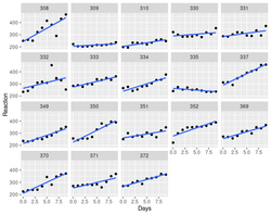
Trajectories
- In longitudinal data analysis, trajectories refer to the patterns of change over time in a variable or set of variables for an individual or group of individuals1. These patterns can be used to identify typical trajectories in longitudinal data using mixed effects models1. The result is summarized in terms of an average trajectory plus measures of the individual variations around this average
- Identifying typical trajectories in longitudinal data: modelling strategies and interpretations 2020
- Visualise longitudinal data
- An example: a model that there are random intercepts and slopes for each subject:
[math]\displaystyle{ y_{ij} = \beta_0 + \beta_1 x_{ij} + b_{0i} + b_{1i} x_{ij} + e_{ij}
}[/math]
- [math]\displaystyle{ y_{ij} }[/math] is the reaction time for subject i at time j
- [math]\displaystyle{ \beta_0, \beta_1 }[/math] are fixed intercept and slope
- [math]\displaystyle{ x_{ij} }[/math] is the number of days since the start of the study for subject i at time j
- [math]\displaystyle{ b_{0i}, b_{1i} }[/math] are the random intercept & slope for subject i
- [math]\displaystyle{ e_{ij} }[/math] is the residual error for subject i at time j
> library(lme4) > data(sleepstudy) # from lme4 > # Fit a mixed effects model with random intercepts and slopes for each subject > model <- lmer(Reaction ~ Days + (Days | Subject), sleepstudy) > > # Plot the fitted model > plot(model, type = "l") > summary(model) Linear mixed model fit by REML ['lmerMod'] Formula: Reaction ~ Days + (Days | Subject) Data: sleepstudy REML criterion at convergence: 1743.6 Scaled residuals: Min 1Q Median 3Q Max -3.9536 -0.4634 0.0231 0.4634 5.1793 Random effects: Groups Name Variance Std.Dev. Corr Subject (Intercept) 612.10 24.741 Days 35.07 5.922 0.07 Residual 654.94 25.592 Number of obs: 180, groups: Subject, 18 Fixed effects: Estimate Std. Error t value (Intercept) 251.405 6.825 36.838 Days 10.467 1.546 6.771 Correlation of Fixed Effects: (Intr) Days -0.138- The fixed effect estimate for Days is 10.4673, which means that on average, reaction times decrease by 10.4673 milliseconds per day.
- The random intercept variance is 612.09, which means that there is considerable variation in the baseline reaction times between subjects.
- The random slope variance is 35.07, which means that there is considerable variation in the rate of change of reaction times over time between subjects.
- It seems no p-values are returned. See Three ways to get parameter-specific p-values from lmer & How to obtain the p-value (check significance) of an effect in a lme4 mixed model?
- To exclude the random slope term, we can use (1 | Subject)
- To exclude the random intercept term, we can use (0 + Days | Subject)
- To exclude the fix intercept term, we can use y ~ -1 + x + (Days | Subject)
library(nlme) model2 <- lme(Reaction ~ Days, random = ~ Days | Subject, data = sleepstudy) > summary(model2) Linear mixed-effects model fit by REML Data: sleepstudy AIC BIC logLik 1755.628 1774.719 -871.8141 Random effects: Formula: ~Days | Subject Structure: General positive-definite, Log-Cholesky parametrization StdDev Corr (Intercept) 24.740241 (Intr) Days 5.922103 0.066 Residual 25.591843 Fixed effects: Reaction ~ Days Value Std.Error DF t-value (Intercept) 251.40510 6.824516 161 36.83853 Days 10.46729 1.545783 161 6.77151 p-value (Intercept) 0 Days 0 Correlation: (Intr) Days -0.138 Standardized Within-Group Residuals: Min Q1 Med Q3 -3.95355735 -0.46339976 0.02311783 0.46339621 Max 5.17925089 Number of Observations: 180 Number of Groups: 18- To exclude the random slope term, we can use random = ~1 | Subject.
- To exclude the random intercept, we can use random = ~Days - 1 | Subject.
Graphical display using facet_wrap().
- lmerTest - Tests in Linear Mixed Effects Models.
The ranova() function in the lmerTest package is used to compute an ANOVA-like table with tests of random-effect terms in a mixed-effects model. Paper in JSS 2017.
# Fixed effect
> anova(model)
Type III Analysis of Variance Table with Satterthwaite's method
     Sum Sq Mean Sq NumDF DenDF F value    Pr(>F)
Days  30031   30031     1    17  45.853 3.264e-06 ***
---
Signif. codes:
0 ‘***’ 0.001 ‘**’ 0.01 ‘*’ 0.05 ‘.’ 0.1 ‘ ’ 1

> anova(model2)
            numDF denDF   F-value p-value
(Intercept)     1   161 1454.0766  <.0001
Days            1   161   45.8534  <.0001

# Random effect
> ranova(model)
ANOVA-like table for random-effects: Single term deletions

Model:
Reaction ~ Days + (Days | Subject)
                         npar  logLik    AIC    LRT Df
<none>                      6 -871.81 1755.6
Days in (Days | Subject)    4 -893.23 1794.5 42.837  2
                         Pr(>Chisq)
<none>
Days in (Days | Subject)   4.99e-10 ***
---
Signif. codes:
0 ‘***’ 0.001 ‘**’ 0.01 ‘*’ 0.05 ‘.’ 0.1 ‘ ’ 1

variancePartition
variancePartition Quantify and interpret divers of variation in multilevel gene expression experiments
Prussian Horse Kicks II example
- Prussian Horse Kicks II: Mixed Effects Models
- In the Prussian horse-kick dataset:
- Each corps = a military unit (like a regiment).
- Each year = a year between 1875–1894.
- The outcome = number of deaths from horse kicks in that corps and year.
- At first glance, we might try a Poisson regression (a GLM): glm(deaths ~ year, family = poisson, data = data). That fits one global trend — the same intercept and slope for everyone.
- Different corps might have different cultures, commanders, or exposure — so some might have more or fewer deaths overall. glm(deaths ~ year + corps, family = poisson, data = data). But this treats corps as fixed effects — separate intercepts for each unit — and that quickly becomes messy when you have dozens or hundreds of groups.
- A mixed-effects model (a.k.a. multilevel or hierarchical model) handles this better by saying: "Each corps has its own intercept (and maybe slope), but those are drawn from a distribution.”
- The model
[math]\displaystyle{
Y_{ij} = \beta_0 + \beta_1 X_{ij} + u_{0j} + u_{1j} X_{ij} + \varepsilon_{ij},
}[/math]
[math]\displaystyle{
\begin{pmatrix}
u_{0j} \\
u_{1j}
\end{pmatrix}
\sim
\text{Normal}
\left(
\begin{pmatrix}
0 \\
0
\end{pmatrix},
\begin{pmatrix}
\sigma_0^2 & \rho\sigma_0\sigma_1 \\
\rho\sigma_0\sigma_1 & \sigma_1^2
\end{pmatrix}
\right),
}[/math]
[math]\displaystyle{
\varepsilon_{ij} \sim \text{Normal}(0, \sigma^2)
}[/math]
The model has 5 parameters total:- 2 fixed effects (intercept and slope),
- 3 random-effect distribution parameters (two variances + one correlation).
- The model in this example
[math]\displaystyle{
Y_{ij} \sim \text{Poisson}(\lambda_{ij}),
}[/math]
[math]\displaystyle{
\log(\lambda_{ij}) = \beta_0 + \beta_1 (\text{Year}_{ij}-\text{midyear)} + u_{0j} + u_{1j}(\text{Year}_{ij} - \text{midyear}),
}[/math]
[math]\displaystyle{
\begin{pmatrix}
u_{0j} \\
u_{1j}
\end{pmatrix}
\sim
\text{Normal}
\left(
\begin{pmatrix}
0 \\
0
\end{pmatrix},
\begin{pmatrix}
\sigma_0^2 & \rho\sigma_0\sigma_1 \\
\rho\sigma_0\sigma_1 & \sigma_1^2
\end{pmatrix}
\right)
}[/math]
where
- i: observation (year)
- j: group (corps)
- u_{0j}: random intercept, u_{1j}: random slope for that corp
- ranef(fit)$corps |> kable(digits = 3) is used to print the estimated random effects (the group-level deviations) for each corps.
- (Intercept): How much this corps’ baseline log death rate differs from the global average.
- I(year-midyear): How much this corps’ time trend (change over years) differs from the global slope.
Growth curve model
Sommer package
- https://cran.r-project.org/web/packages/sommer/index.html Solving Mixed Model Equations in R
- Dealing with correlation in designed field experiments: part II
GEE/generalized estimating equations
- https://en.wikipedia.org/wiki/Generalized_estimating_equation
- Literatures:
- Longitudinal Data Analysis for Discrete and Continuous Outcomes Scott L. Zeger and Kung-Yee Liang Biometrics 1986
- Longitudinal data analysis using generalized linear models. Liang, K., and S. L. Zeger (1986) Biometrika.
- Analysis of Longitudinal Data (Oxford Statistical Science Series) 2nd edition by Peter Diggle, Patrick Heagerty, Kung-Yee Liang, and Scott Zeger
- Youtube
- 12.1 - Introduction to Generalized Estimating Equations from PennState
- 12.2 - Modeling Binary Clustered Responses which shows the "exchangeable" correlation structure
- gee package. First version 1999.
- geepack package. First version 2002.
- Getting Started with Generalized Estimating Equations.
- The Working correlation matrix output from the gee() function when "exchangeable" correlation was used. The dimension of "working correlation" is the number of observations per subject/id. Question: why the diagonal elements of the working correlation is sometimes 0 instead of 1 in my data.
- The Estimated Scale Parameter is the dispersion parameter.
- **A review of Longitudinal Data Analysis in R.
- **DEM 7283: Longitudinal Models for Change using Generalized Estimating Equations
- Chapter 15 GEE, Binary Outcome: Respiratory Illness from Encyclopedia of Quantitative Methods in R, vol. 5: Multilevel Models.
- SAS/STAT 14.1 User’s Guide The GEE Procedure. We can download the data and compare it with the results from R.
- Fast Pure R Implementation of GEE: Application of the Matrix Package
- One example
library(geepack)

# load data
data("cbpp", package = "lme4")
cbpp[1:3, ]
#   herd incidence size period
# 1    1         2   14      1
# 2    1         3   12      2
# 3    1         4    9      3
with(cbpp, table(herd, period))
    period
herd 1 2 3 4
  1  1 1 1 1
  2  1 1 1 0
  3  1 1 1 1
  4  1 1 1 1
  5  1 1 1 1
  6  1 1 1 1
  7  1 1 1 1
  8  1 0 0 0
  9  1 1 1 1
  10 1 1 1 1
  11 1 1 1 1
  12 1 1 1 1
  13 1 1 1 1
  14 1 1 1 1
  15 1 1 1 1

# fit GEE model with logit link
fit <- geeglm(cbind(incidence, size - incidence) ~ period, id = herd,
              family = binomial("logit"), corstr = "exchangeable", data = cbpp)

# summary of the model
summary(fit)
 Coefficients:
            Estimate Std.err  Wald Pr(>|W|)
(Intercept)   -1.270   0.276 21.24  4.0e-06 ***
period2       -1.156   0.436  7.04   0.0080 **
period3       -1.284   0.491  6.84   0.0089 **
period4       -1.754   0.375 21.85  2.9e-06 ***
---
Signif. codes:
0 ‘***’ 0.001 ‘**’ 0.01 ‘*’ 0.05 ‘.’ 0.1 ‘ ’ 1

Correlation structure = exchangeable
Estimated Scale Parameters:

            Estimate Std.err
(Intercept)    0.134  0.0542
  Link = identity

Estimated Correlation Parameters:
      Estimate Std.err
alpha   0.0414   0.129
Number of clusters:   15  Maximum cluster size: 4

summary(fit)$coefficients
            Estimate Std.err  Wald Pr(>|W|)
(Intercept)    -1.27   0.276 21.24 4.04e-06
period2        -1.16   0.436  7.04 7.99e-03
period3        -1.28   0.491  6.84 8.90e-03
period4        -1.75   0.375 21.85 2.94e-06

# extract robust variance-covariance matrix
vcov_fit <- vcovHC(fit, type = "HC")

# compute confidence intervals for coefficients
library(sandwich)

vcov_fit <- vcovHC(fit, type = "HC")
ci <- coef(fit) + cbind(qnorm(0.025), qnorm(0.975)) * sqrt(diag(vcov_fit))
colnames(ci) <- c("2.5 %", "97.5 %")
print(ci)
Compare with gee()
summary(gee(cbind(incidence, size - incidence) ~ period, id = herd, family = binomial("logit"), corstr = "exchangeable", data = cbpp))
# Coefficients:
#             Estimate Naive S.E. Naive z Robust S.E. Robust z
# (Intercept)    -1.27      0.214   -5.94       0.275    -4.61
# period2        -1.16      0.424   -2.74       0.437    -2.66
# period3        -1.29      0.455   -2.83       0.492    -2.62
# period4        -1.76      0.600   -2.94       0.379    -4.65
#
# Estimated Scale Parameter:  2.18
# Number of Iterations:  2
#
# Working Correlation
#        [,1]   [,2]   [,3]   [,4]
# [1,] 1.0000 0.0274 0.0274 0.0274
# [2,] 0.0274 1.0000 0.0274 0.0274
# [3,] 0.0274 0.0274 1.0000 0.0274
# [4,] 0.0274 0.0274 0.0274 1.0000
[math]\displaystyle{ \operatorname{logit}\left(\frac{p_{ij}}{1 - p_{ij}}\right) = \beta_0 + \beta_1 \cdot \text{period}_{ij} + u_j }[/math] where [math]\displaystyle{ p_{ij} }[/math] is the probability of a positive outcome (i.e., an incidence) for
- the [math]\displaystyle{ i }[/math]-th animal/observation in herd(group/subject) [math]\displaystyle{ j }[/math], and
- [math]\displaystyle{ \text{period}_{ij} }[/math] is a categorical predictor variable indicating the period of observation for herd/subject [math]\displaystyle{ j }[/math] and observation [math]\displaystyle{ i }[/math].
- The parameters [math]\displaystyle{ \beta_0 }[/math] and [math]\displaystyle{ \beta_1 }[/math] represent the intercept and the effect of the period variable, respectively.
- The [math]\displaystyle{ u_j }[/math] is the random subject-specific effect. The random effects [math]\displaystyle{ u_j }[/math] are assumed to follow a multivariate normal distribution with mean 0 and covariance matrix [math]\displaystyle{ \Sigma }[/math].
- The correlation structure of the random effects is specified as "exchangeable", which means that any two random effects from the same subject have the same correlation.
R packages
Sort by sample ID & time first
- No effect of corstr argument on correlation structure in gee
- The issue applies to both the gee and geepack packages.
- If observations were not ordered according to cluster and time within cluster we would get the wrong result. See geepack vignette.
- See the section 4 for a case that data is ordered according to subject but the time ordering within subject is random.
- For the depression data from Getting Started with Generalized Estimating Equations, data are sorted by id & time. It is also true for dietox data included in geepack: all(order(dietox$Pig, dietox$Time) == 1:nrow(dietox)) = TRUE.
- Both geeglm() or gee() does not require a 'time' parameter because it assumes the time is sorted within a cluster. But how about data has missing values?
- Do unequal time intervals for waves parameter in gee analysis matter? (geeglm in R) no answer.
- Use the "waves" parameter. waves specifying the ordering of repeated mesurements on the same unit. Also used in connection with missing values. See the vignette.
- waves names a positive integer-valued variable that is used to identify the order and spacing of observations within groups in a GEE model. This argument is crucial when there are missing values and gaps in the data. See examples on Lecture 23 (lab 8)—Friday, March 2, 2012.
- "waves" is only available in geeglm(). It is not available in gee().
Compare models
- 015. GEE in Practice: Example on COVID-19 Test Positivity Data. QIC is available in the geepack package.
- geeglm was used.
- simple scatterplot by plot() with y=positivity_rate, x=time
- lattice::xyplot()
xyplot(positivity_rate ~ time|ID,
       groups = ID,
       subset = ID %in% sampled_idx,
       data= covid,
       panel = function(x, y) {
         panel.xyplot(x, y, plot='p')
         panel.linejoin(x, y,
                       fun=mean,
                       horizontal = F,
                       lwd=2, col=1)
       })
- create a factor
covid$size_factor <-  cut(covid$estimat_pop,
                   breaks = quantile(unique(covid$estimated_pop)),
                   include.lowest = TRUE,
                   lables = FALSE)  |>  as.factor()

xyplot(positivity_rate ~ time|size_factor, # size_factor is like a facet
       groups = ID,
       data= covid,
       panel = function(x, y) {
         panel.xyplot(x, y, plot='p')
         panel.linejoin(x, y,
                       fun=mean,
                       horizontal = F,
                       lwd=2, col=1)
       })
- Residual vs predict plot from plot(fit) can be used to evaluate which correlation structure is better.
- QIC() output and what metric can be used for [model selection. QIC & CIC are most useful for selecting correlation structure. QICU is most useful for comparing models with the same correlation structure but different mean structure.
- Analysis of panel data in R using Generalized Estimating Equations which uses the MESS package
anova()
anova() method works on geeglm() object but not on gee() object.
Simulation
- How to simulate data for generalized estimating equations (GEE) with logistic link function?
- We generate some example data with repeated measurements. In this simulated data, we have 100 subjects, each measured at 5 time points.
# Load the geepack package
library(geepack)

# Generate some example data with repeated measurements
set.seed(123)
n <- 100  # Number of subjects
time <- rep(1:5, each = n)  # Time points
subject <- rep(1:n, times = 5)  # Subject IDs
y <- rnorm(n * 5, mean = time * 0.5 + subject * 0.2)  # Simulated response variable

# Create a data frame
data <- data.frame(subject, time, y)
data <- data[order(data$subject, data$time), ]
data[1:4, ]
#     subject time      y
# 1         1    1 0.1395
# 101       1    2 0.4896
# 201       1    3 3.8988
# 301       1    4 1.4848

# Fit a GEE model using geeglm
# In this example, we assume an exchangeable correlation structure
model <- geeglm(y ~ time, id = subject, data = data, family = gaussian, corstr = "exchangeable")

# Summary of the GEE model
summary(model)
#  Coefficients:
#             Estimate Std.err Wald Pr(>|W|)
# (Intercept)   10.104   0.594  289   <2e-16 ***
# time           0.510   0.033  240   <2e-16 ***
# ---
# Signif. codes:  0 ‘***’ 0.001 ‘**’ 0.01 ‘*’ 0.05 ‘.’ 0.1 ‘ ’ 1
#
# Correlation structure = exchangeable
# Estimated Scale Parameters:
#
#             Estimate Std.err
# (Intercept)     35.1    3.07
#   Link = identity
#
# Estimated Correlation Parameters:
#       Estimate Std.err
# alpha    0.972 0.00333               ===> corr estimate is 0.972
# Number of clusters:   100  Maximum cluster size: 5

model2 = geeglm(y ~ time, id = subject, data = data, family = gaussian, corstr = "ind")
summary(model2)
#  Coefficients:
#             Estimate Std.err Wald Pr(>|W|)
# (Intercept)   10.104   0.594  289   <2e-16 ***
# time           0.510   0.033  240   <2e-16 ***
# ---
# Signif. codes:  0 ‘***’ 0.001 ‘**’ 0.01 ‘*’ 0.05 ‘.’ 0.1 ‘ ’ 1
#
# Correlation structure = independence
# Estimated Scale Parameters:
#
#             Estimate Std.err
# (Intercept)     35.1    3.07
# Number of clusters:   100  Maximum cluster size: 5

# gee() from gee package
summary(gee(y ~ time, id = subject, data = data, family = gaussian, corstr = "exchangeable"))
# Coefficients:
#             Estimate Naive S.E. Naive z Robust S.E. Robust z
# (Intercept)    10.10     0.5945    17.0       0.594     17.0
# time            0.51     0.0327    15.6       0.033     15.5
#
# Estimated Scale Parameter:  35.2
# Number of Iterations:  1
#
# Working Correlation
#      [,1] [,2] [,3] [,4] [,5]
# [1,] 1.00 0.97 0.97 0.97 0.97
# [2,] 0.97 1.00 0.97 0.97 0.97
# [3,] 0.97 0.97 1.00 0.97 0.97
# [4,] 0.97 0.97 0.97 1.00 0.97
# [5,] 0.97 0.97 0.97 0.97 1.00
gee vs glm
# See the next subsection about dietox dataset
glmEx <- glm(mf, data=dietox, family=gaussian)
> summary(glmEx)

Call:
glm(formula = mf, family = gaussian, data = dietox)

Coefficients:
            Estimate Std. Error t value             Pr(>|t|)
(Intercept)   15.073      0.709   21.27 < 0.0000000000000002 ***
Time           6.948      0.069  100.66 < 0.0000000000000002 ***
EvitEvit100    2.081      0.589    3.54              0.00043 ***
EvitEvit200   -1.113      0.582   -1.91              0.05619 .
CuCu035       -0.789      0.583   -1.35              0.17638
CuCu175        1.777      0.589    3.02              0.00264 **
---
Signif. codes:  0 ‘***’ 0.001 ‘**’ 0.01 ‘*’ 0.05 ‘.’ 0.1 ‘ ’ 1

(Dispersion parameter for gaussian family taken to be 48.62)

    Null deviance: 536592  on 860  degrees of freedom
Residual deviance:  41571  on 855  degrees of freedom
AIC: 5796

Number of Fisher Scoring iterations: 2
In this particular instance, the application of linear regression yields a lower standard error (SE) for each variable when compared to the Generalized Estimating Equations (GEE) method. In other words, linear regression assumes that all observations are independent. If this assumption is violated, as is often the case with longitudinal data where measurements from the same subject over time are likely to be correlated, the standard errors produced by linear regression may be underestimated. This could lead to overly optimistic p-values and confidence intervals that do not cover the true parameter value as often as they should.
gee vs geepack packages
GENERALIZED ESTIMATING EQUATIONS (GEE) by Practical Statistics (Rebecca Barter).
Subject-specific versus Population-averaged.
GEE estimates population-averaged model parameters and their standard errors.
library("geepack")
data(dietox)
dietox$Cu <- as.factor(dietox$Cu)
dietox$Evit <- as.factor(dietox$Evit)
mf <- formula(Weight ~ Time + Evit + Cu)

geeEx <- geeglm(mf, id=Pig, data=dietox, family=gaussian, corstr="ex")
summary(geeEx)

Call:
geeglm(formula = mf, family = gaussian, data = dietox, id = Pig,
    corstr = "ex")

 Coefficients:
            Estimate Std.err    Wald Pr(>|W|)
(Intercept)  15.0984  1.4206  112.96   <2e-16 ***
Time          6.9426  0.0796 7605.79   <2e-16 ***
EvitEvit100   2.0414  1.8431    1.23     0.27
EvitEvit200  -1.1103  1.8452    0.36     0.55
CuCu035      -0.7652  1.5354    0.25     0.62
CuCu175       1.7871  1.8189    0.97     0.33
---
Signif. codes:  0 ‘***’ 0.001 ‘**’ 0.01 ‘*’ 0.05 ‘.’ 0.1 ‘ ’ 1

Correlation structure = exchangeable
Estimated Scale Parameters:

            Estimate Std.err
(Intercept)     48.3    9.31
  Link = identity

Estimated Correlation Parameters:
      Estimate Std.err
alpha    0.766  0.0326
Number of clusters:   72  Maximum cluster size: 12
Note that the correlation estimate obtained from geeglm() is 0.766 = summary(geeEx)$geese$correlation$estimate.
gee() can show the complete correlation structure in the output. The correlation estimate is 0.761 =summary(geeEx2)$working.correlation[1, 2].
geeEx2 = gee::gee(Weight ~ Time + Evit + Cu, id=Pig, data=dietox, family=gaussian, corstr="exchangeable")
summary(geeEx2)
Beginning Cgee S-function, @(#) geeformula.q 4.13 98/01/27
running glm to get initial regression estimate
(Intercept)        Time EvitEvit100 EvitEvit200     CuCu035     CuCu175
     15.073       6.948       2.081      -1.113      -0.789       1.777

 GEE:  GENERALIZED LINEAR MODELS FOR DEPENDENT DATA
 gee S-function, version 4.13 modified 98/01/27 (1998)

Model:
 Link:                      Identity
 Variance to Mean Relation: Gaussian
 Correlation Structure:     Exchangeable

Call:
gee::gee(formula = Weight ~ Time + Evit + Cu, id = Pig, data = dietox,
    family = gaussian, corstr = "exchangeable")

Summary of Residuals:
    Min      1Q  Median      3Q     Max
-34.396  -3.245   0.903   4.127  20.157


Coefficients:
            Estimate Naive S.E. Naive z Robust S.E. Robust z
(Intercept)   15.098     1.6955   8.905      1.4206   10.628
Time           6.943     0.0337 205.820      0.0796   87.211
EvitEvit100    2.041     1.7991   1.135      1.8431    1.108
EvitEvit200   -1.110     1.7813  -0.623      1.8452   -0.602
CuCu035       -0.765     1.7813  -0.430      1.5354   -0.498
CuCu175        1.787     1.7991   0.993      1.8189    0.982

Estimated Scale Parameter:  48.6
Number of Iterations:  2

Working Correlation
       [,1]  [,2]  [,3]  [,4]  [,5]  [,6]  [,7]  [,8]  [,9] [,10] [,11] [,12]
 [1,] 1.000 0.761 0.761 0.761 0.761 0.761 0.761 0.761 0.761 0.761 0.761 0.761
 [2,] 0.761 1.000 0.761 0.761 0.761 0.761 0.761 0.761 0.761 0.761 0.761 0.761
 [3,] 0.761 0.761 1.000 0.761 0.761 0.761 0.761 0.761 0.761 0.761 0.761 0.761
 [4,] 0.761 0.761 0.761 1.000 0.761 0.761 0.761 0.761 0.761 0.761 0.761 0.761
 [5,] 0.761 0.761 0.761 0.761 1.000 0.761 0.761 0.761 0.761 0.761 0.761 0.761
 [6,] 0.761 0.761 0.761 0.761 0.761 1.000 0.761 0.761 0.761 0.761 0.761 0.761
 [7,] 0.761 0.761 0.761 0.761 0.761 0.761 1.000 0.761 0.761 0.761 0.761 0.761
 [8,] 0.761 0.761 0.761 0.761 0.761 0.761 0.761 1.000 0.761 0.761 0.761 0.761
 [9,] 0.761 0.761 0.761 0.761 0.761 0.761 0.761 0.761 1.000 0.761 0.761 0.761
[10,] 0.761 0.761 0.761 0.761 0.761 0.761 0.761 0.761 0.761 1.000 0.761 0.761
[11,] 0.761 0.761 0.761 0.761 0.761 0.761 0.761 0.761 0.761 0.761 1.000 0.761
[12,] 0.761 0.761 0.761 0.761 0.761 0.761 0.761 0.761 0.761 0.761 0.761 1.000
and we need to calculate p-values manually.
> format.pval(2*(1-pnorm(abs(summary(geeEx2)$coefficients[, "Robust z"]))))
[1] "< 2e-16" "< 2e-16" "0.26804" "0.54737" "0.61823" "0.32585"
GEE vs. mixed effects models
- When to use generalized estimating equations vs. mixed effects models?
- GEE fits a marginal regression model to the longitudinal data.
- Instead of attempting to model the within-subject covariance structure, GEE models the average response. The goal is to make inferences about the population when accounting for the within-subject correlation. For every one-unit increase in a covariate across the population, GEE tells us how much the average response would change.
- GEE can take into account the correlation of within-subject data (longitudinal studies) and other studies in which data are clustered within subgroups. Failure to take into account correlation would lead to the regression estimates (Bs) being less efficient, meaning they would be more widely scattered around the true population value.
- GEE fits a marginal model, which means it models the average response over time, rather than modeling each individual's response over time. This is different from other methods like mixed-effects models, which model both the population average and individual deviations from that average.
- The advantage of using a marginal model is that it provides a simpler interpretation of the results. The regression coefficients from a GEE model represent the average change in the response for a one-unit change in the predictor, averaged over all individuals in the population. This can be easier to interpret and communicate than individual-level effects.
- Moreover, GEE is less sensitive to misspecification of the correlation structure compared to other methods. This means that even if you don't correctly specify how the repeated measurements are correlated, you can still get valid estimates of the average effects. That is, GEE is robust to misspecification of the within-subject correlation.
- Mixed-effects models, on the other hand, provide an individual-level approach by adopting random effects to capture the correlation between the observations of the same subject. They give an interpretation conditional on the random effects.
- The fundamental difference between GEE and mixed-effects models lies in the interpretation of the coefficients. GEEs produce population-averaged effects, while mixed-effects models produce subject-specific effects. In other words, GEEs give you the more usual interpretation of comparing groups of subjects, while mixed-effects models give an interpretation conditional on the random effects.
- For example, consider a binary outcome with a logit link. The GEE would give you the log-odds ratio between groups (e.g., males vs. females), which is a population-averaged effect. On the other hand, a mixed-effects model would give you an estimate that accounts for individual-specific random effects.
- In summary, whether to use GEE or a mixed-effects model depends on your research question and whether you are interested in population-averaged or subject-specific effects.
- https://stats.stackexchange.com/a/16415
- Getting Started with Generalized Estimating Equations
- It uses "gee", "lme4", "geepack" packages for model fittings
dep_gee2 <- gee(depression ~ diagnose + drug*time, data = dat, id = id, family = binomial, corstr = "exchangeable")- How does the GEE model with the exchangeable correlation structure compare to a Generalized Mixed-Effect model. We allow the intercept to be conditional on subject. This means we’ll get 340 subject_specific models with different intercepts but identical coefficients for everything else. The model coefficients listed under “Fixed effects” are almost identical to the GEE coefficients. ?glmer for GLMMs/Generalized Linear Mixed-Effects Models.
library(lme4) # version 1.1-31
dep_glmer <- glmer(depression ~ diagnose + drug*time + (1|id),
               data = dat, family = binomial)
summary(dep_glmer, corr = FALSE)
dep_gee4 <- geeglm(depression ~ diagnose + drug*time, data = dat, id = id, family = binomial, corstr = "exchangeable")
- "ggeffects" package for plotting. The emmeans function calculates marginal effects and works for both GEE and mixed-effect models.
library(ggeffects)
library(emmeans)
plot(ggemmeans(dep_glmer, terms = c("time", "drug"),
               condition = c(diagnose = "severe"))) +
  ggplot2::ggtitle("GLMER Effect plot")

data.frame(ggemmeans(dep_glmer, terms = c("time", "drug"),
           condition = c(diagnose = "severe")) )
  x predicted std.error conf.low conf.high    group
1 0     0.207     0.175    0.156     0.269 standard
2 0     0.197     0.187    0.146     0.262      new
3 1     0.297     0.119    0.251     0.348 standard
4 1     0.525     0.126    0.463     0.586      new
5 2     0.407     0.156    0.335     0.482 standard
6 2     0.832     0.217    0.764     0.883      new
filter(dat, diagnose == "severe") %>%
   group_by(drug, time) %>%
   summarize(mean = mean(depression))
  drug      time  mean
  <fct>    <int> <dbl>
1 standard     0 0.21
2 standard     1 0.28
3 standard     2 0.46
4 new          0 0.178
5 new          1 0.5
6 new          2 0.833

plot(ggemmeans(dep_gee4, terms = c("time", "drug"),
               condition = c(diagnose = "severe"))) +
  ggplot2::ggtitle("GEE Effect plot")
- While both methods are used for modeling correlated data, there are some key differences between them.
- Assumptions: The key difference between GEE and nlme is that GEE makes fewer assumptions about the underlying data structure. GEE assumes that the mean structure is correctly specified, but the correlation structure is unspecified. In contrast, nlme assumes that both the mean and the variance-covariance structure are correctly specified.
- Model flexibility: GEE is a more flexible model than nlme because it allows for modeling the mean and variance of the response separately. This means that GEE is more suitable for modeling data with non-normal errors, such as count or binary data. In contrast, nlme assumes that the errors are normally distributed and allows for modeling the mean and variance jointly.
- Inference: Another key difference between GEE and nlme is the type of inference they provide. GEE provides marginal inference, which means that it estimates the population-averaged effect of the predictor variables on the response variable. In contrast, nlme provides conditional inference, which means that it estimates the subject-specific effect of the predictor variables on the response variable.
- Computation: The computation involved in fitting GEE and nlme models is also different. GEE uses an iterative algorithm to estimate the model parameters, while nlme uses a maximum likelihood estimation approach. The computational complexity of GEE is lower than that of nlme, making it more suitable for large datasets.
- In summary, GEE and nlme are two popular models used for analyzing longitudinal data. The main differences between the two models are the assumptions they make, model flexibility, inference type, and computational complexity. GEE is a more flexible model that makes fewer assumptions and provides marginal inference, while nlme assumes normality of errors and provides conditional inference.
Independent correlation
If you assume an independent correlation structure in a Generalized Estimating Equation (GEE) model, the GEE estimates are the same as those obtained from a Generalized Linear Model (GLM) or Ordinary Least Squares (OLS) if the dependent variable is normally distributed and no correlation within responses are assumed².
However, the standard errors in a GEE model will be different from those in a GLM or OLS model. This is because GEE takes into account the within-subject correlation, which can lead to more efficient estimates¹. If this correlation is not taken into account, the regression estimates would be less efficient, meaning they would be more widely scattered around the true population value¹.
It's important to note that while the point estimates might be the same, the interpretation of these estimates differs between GEE and GLM/OLS models. In a GEE model, you're making inferences about the population average response, whereas in a GLM/OLS model, you're making inferences about individual-level effects¹.
References:
- GEE: choosing proper working correlation structure.
- GEE for Repeated Measures Analysis | Columbia Public Health.
exchangeable correlation
- It seems geeglm() and gee() can return different estimate of correlation.
- For geeglm(), we can find the estimate from the summary output. See an example (0.3285) below.
Estimated Correlation Parameters:
      Estimate Std.err
alpha   0.3285 0.08381
SAS
The GEE procedure - Example 50.1 Comparison of the Marginal and Random Effect Models for Binary Data. The data (& the code) can be downloaded from this link. A copy of the data is available at github.
Note the data has been sorted by subject ("centerid") and time ("visit") within each subject. The data has no missing values. So there is no need to use the waves parameter.
library(geepack)
library(gee)

resp <- read.table("~/Downloads/resp.txt", header = T)
> dim(resp)
[1] 111  10
> resp[1:2, ]
  center id treat sex age baseline visit1 visit2 visit3 visit4
1      1  1     P   M  46        0      0      0      0      0
2      1  2     P   M  28        0      0      0      0      0

library(tidyr)
resp.long <- pivot_longer(resp, starts_with("visit"), names_to = 'n', values_to = 'v'))
resp.long <- mutate(resp.long, centerid = center*id)
R> resp.long[1:3, ]
# A tibble: 3 × 9
  center    id treat sex     age baseline n          v centerid
   <int> <int> <chr> <chr> <int>    <int> <chr>  <int>    <int>
1      1     1 P     M        46        0 visit1     0        1
2      1     1 P     M        46        0 visit2     0        1
3      1     1 P     M        46        0 visit3     0        1
resp.long <- mutate(resp.long, center = as.factor(center), treat = as.factor(treat),
                    sex = as.factor(sex), baseline = factor(baseline))

> mod = geeglm(v~ treat + center + sex + age + baseline, family=binomial, data=resp.long,
 			id=centerid, corstr="exch")
> summary(mod)

Call:
geeglm(formula = v ~ treat + center + sex + age + baseline, family = binomial,
    data = resp.long, id = centerid, corstr = "exch")

 Coefficients:
            Estimate  Std.err   Wald Pr(>|W|)
(Intercept)  0.54603  0.72348  0.570 0.450416
treatP      -1.26536  0.34668 13.322 0.000262 ***
center2      0.64949  0.35322  3.381 0.065952 .
sexM        -0.13678  0.44025  0.097 0.756035
age         -0.01876  0.01296  2.093 0.147974
baseline1    1.84572  0.34598 28.460 9.57e-08 ***
---
Signif. codes:  0 ‘***’ 0.001 ‘**’ 0.01 ‘*’ 0.05 ‘.’ 0.1 ‘ ’ 1

Correlation structure = exchangeable
Estimated Scale Parameters:

            Estimate Std.err
(Intercept)    1.002  0.1842
  Link = identity

Estimated Correlation Parameters:
      Estimate Std.err
alpha   0.3285 0.08381
Number of clusters:   111  Maximum cluster size: 4

> mod2 = gee(v~ treat + center + sex + age + baseline, family=binomial, data=resp.long,
  id=centerid, corstr="exchangeable")
Beginning Cgee S-function, @(#) geeformula.q 4.13 98/01/27
running glm to get initial regression estimate
(Intercept)      treatP     center2        sexM         age   baseline1
    0.54603    -1.26536     0.64949    -0.13678    -0.01876     1.84572
> summary(mod2)
Coefficients:
            Estimate Naive S.E. Naive z Robust S.E. Robust z
(Intercept)  0.54603     0.6585  0.8292     0.72348   0.7547
treatP      -1.26536     0.3333 -3.7962     0.34668  -3.6499
center2      0.64949     0.3379  1.9219     0.35322   1.8388
sexM        -0.13678     0.4161 -0.3288     0.44025  -0.3107
age         -0.01876     0.0125 -1.5000     0.01296  -1.4467
baseline1    1.84572     0.3394  5.4386     0.34598   5.3348

Estimated Scale Parameter:  1.016
Number of Iterations:  1

Working Correlation
      [,1]  [,2] [,3] [,4] [,5] [,6] [,7] [,8]
[1,] 1.000 0.327    0    0    0    0    0    0
[2,] 0.327 0.327    0    0    0    0    0    0
[3,] 0.327 1.000    0    0    0    0    0    0
[4,] 0.327 0.327    0    0    0    0    0    0
[5,] 0.327 0.327    0    0    0    0    0    0
[6,] 1.000 0.327    0    0    0    0    0    0
[7,] 0.327 0.327    0    0    0    0    0    0
[8,] 0.327 1.000    0    0    0    0    0    0