File list
Jump to navigation
Jump to search
This special page shows all uploaded files.
| Date | Name | Thumbnail | Size | User | Description | Versions |
|---|---|---|---|---|---|---|
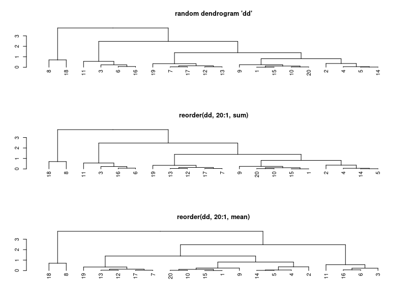
| 12:15, 8 January 2023 | Reorder.dendrogram.png (file) |  |
10 KB | Brb | <pre> set.seed(123) x <- rnorm(20) hc <- hclust(dist(x)) dd <- as.dendrogram(hc) par(mfrow=c(3, 1)) plot(dd, main = "random dendrogram 'dd'") # not the same as reorder(dd, 1:20) plot(reorder(dd, 20:1), main = 'reorder(dd, 20:1, sum)') plot(reorder(dd, 20:1, mean), main = 'reorder(dd, 20:1, mean)') </pre> | 1 |
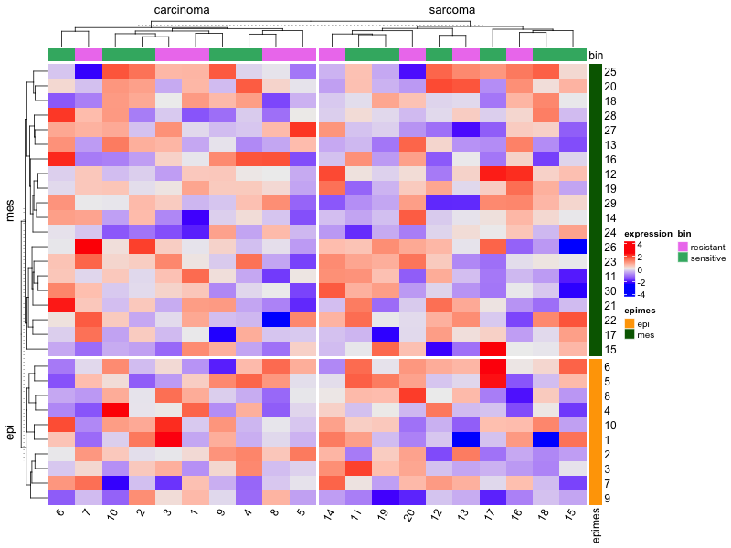
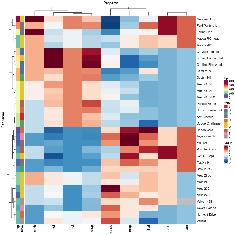
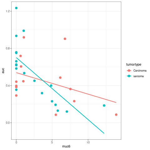
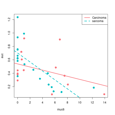
| 21:37, 7 January 2023 | ComplexHeatmap2.png (file) |  |
43 KB | Brb | <syntaxhighlight lang="rsplus"> # Simulate data library(ComplexHeatmap) ng <- 30; ns <- 20 set.seed(1) mat <- matrix(rnorm(ng*ns), nr=ng, nc=ns) colnames(mat) <- 1:ns rownames(mat) <- 1:ng # color bar on RHS ind_e <- 1:round(ng/3) ind_m <- (1+round(ng/3)):ng epimes <- rep(c("epi", "mes"), c(length(ind_e), length(ind_m))) row_ha <- rowAnnotation(epimes = epimes, col = list(epimes = c("epi" = "orange", "mes" = "darkgreen"))) # color bar on Top tumortype <- rep(c("carcinoma", "sarcoma"... | 1 |
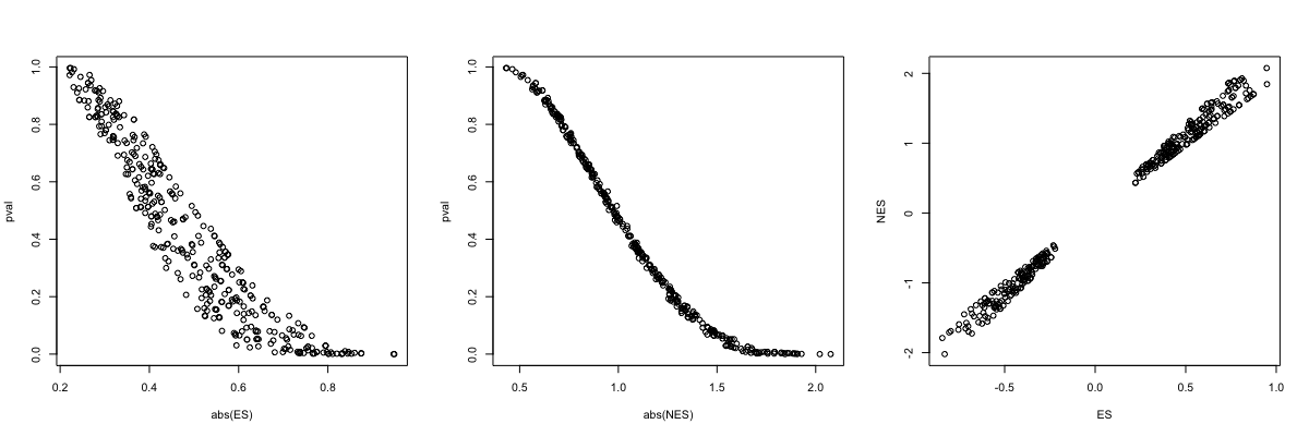
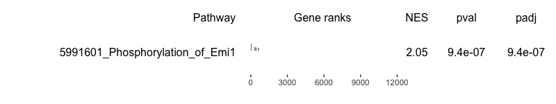
| 12:37, 6 January 2023 | Fgsea3plots.png (file) |  |
68 KB | Brb | <pre> par(mfrow=c(1,3)) with(fgseaRes, plot(abs(ES), pval)) with(fgseaRes, plot(abs(NES), pval)) with(fgseaRes, plot(ES, NES)) </pre> | 1 |
| 14:58, 31 December 2022 | Filebrowser.png (file) |  |
86 KB | Brb | 1 | |
| 20:07, 25 December 2022 | DisableDropbox4pm.png (file) |  |
246 KB | Brb | 1 | |
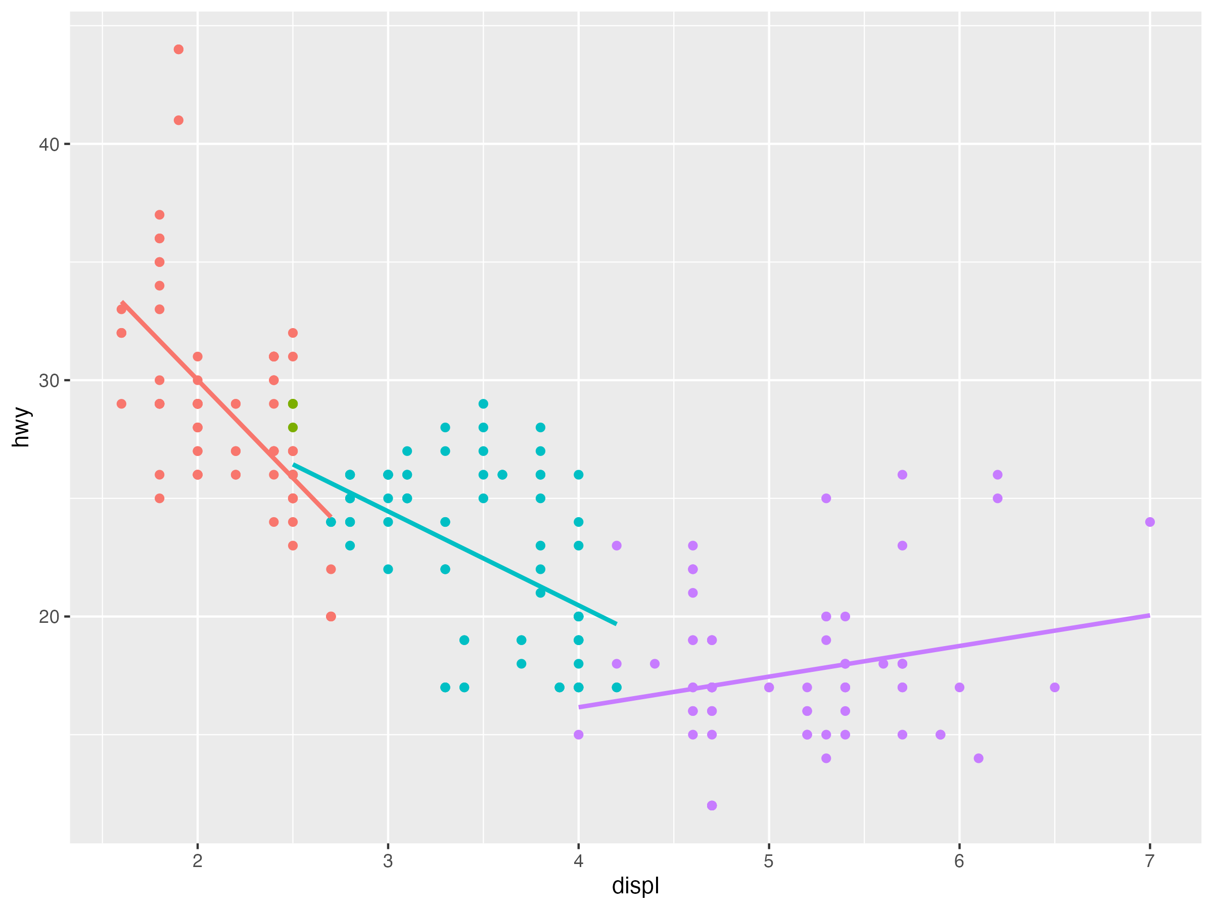
| 15:40, 15 December 2022 | Geom smooth ex.png (file) |  |
110 KB | Brb | <pre> library(dplyr) #group the data by cyl and create the plots mpg %>% group_by(cyl) %>% ggplot(aes(x=displ, y=hwy, color=factor(cyl))) + geom_point() + geom_smooth(method = "lm", se = FALSE) + theme(legend.position="none") </pre> | 1 |
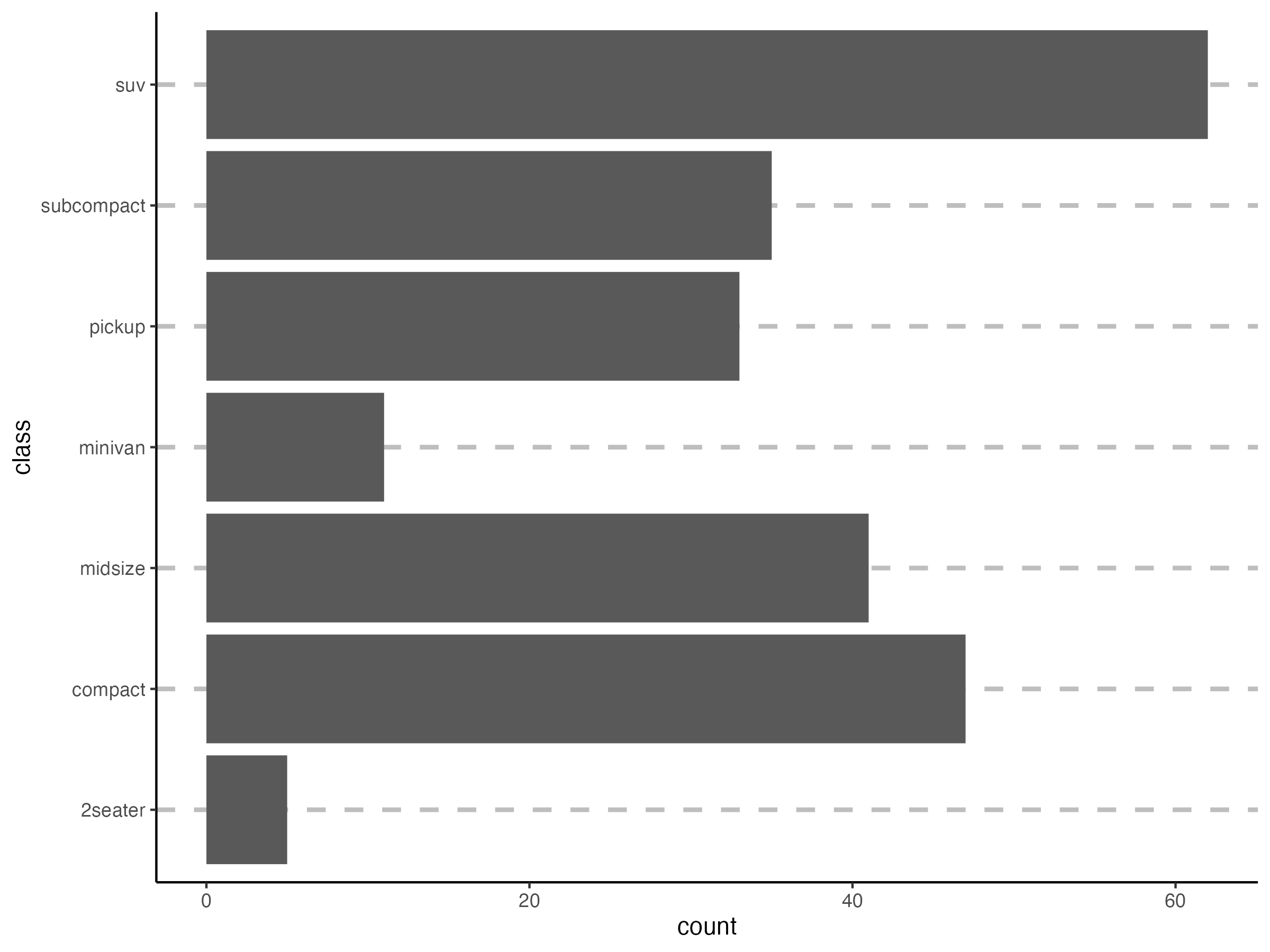
| 15:14, 15 December 2022 | Geom bar4.png (file) |  |
51 KB | Brb | <pre> ggplot(mpg, aes(x = class)) + geom_vline(xintercept = mpg$class, color = "grey", linetype = "dashed", size = 1) + geom_bar() + theme_classic() + coord_flip() </pre> | 1 |
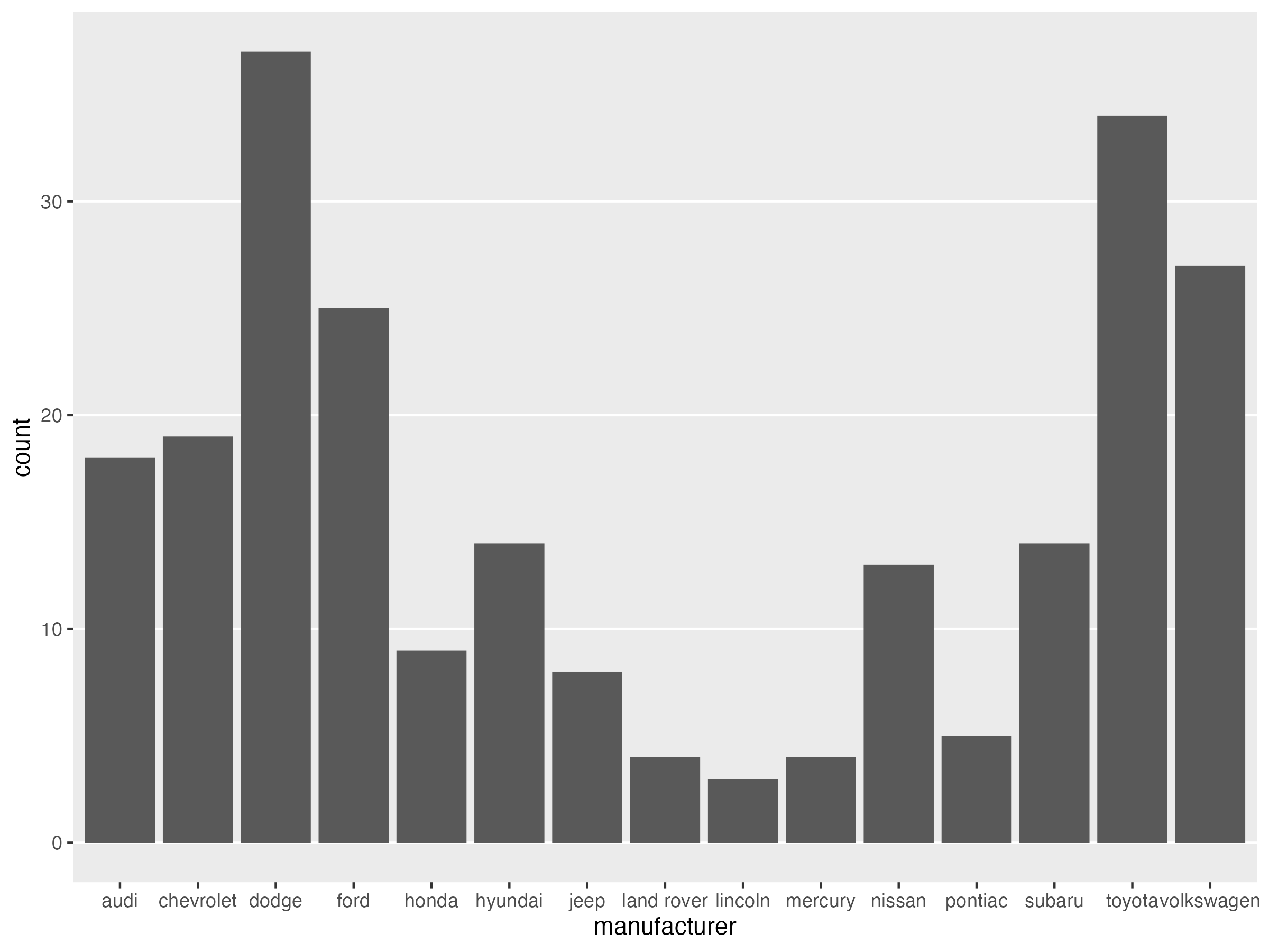
| 15:08, 15 December 2022 | Geom bar3.png (file) |  |
44 KB | Brb | <pre> ggplot(mpg, aes(x=manufacturer)) + geom_bar() + theme(panel.grid.major.x = element_blank(), panel.grid.minor = element_blank()) </pre> | 1 |
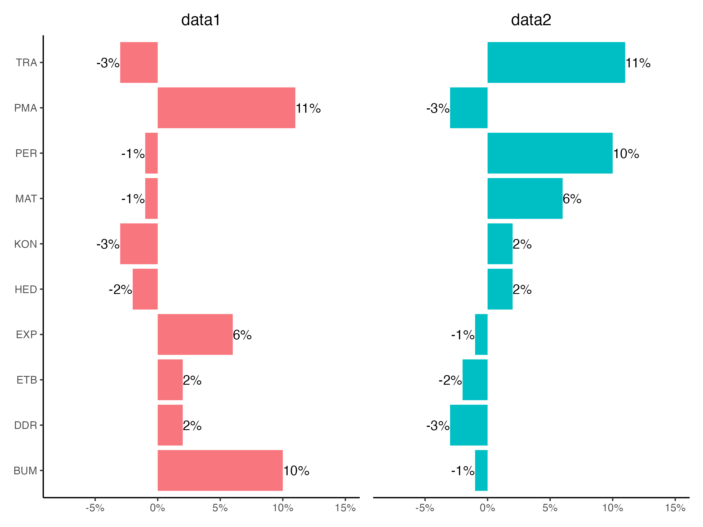
| 14:41, 15 December 2022 | Geom bar2.png (file) |  |
71 KB | Brb | <pre> library(ggplot2) library(scales) library(patchwork) dtf <- data.frame(x = c("ETB", "PMA", "PER", "KON", "TRA", "DDR", "BUM", "MAT", "HED", "EXP"), y = c(.02, .11, -.01, -.03, -.03, .02, .1, -.01, -.02, 0.06)) set.seed(1) dtf2 <- data.frame(x = dtf[, 1], y = sample(dtf[, 2])) g1 <- ggplot(dtf, aes(x, y)) + geom_bar(stat = "identity", fill = "#F8767D") + geom_text(aes(label = paste0(y * 100, "%"), hjust = ifelse(y >= 0, 0, 1))) +... | 1 |
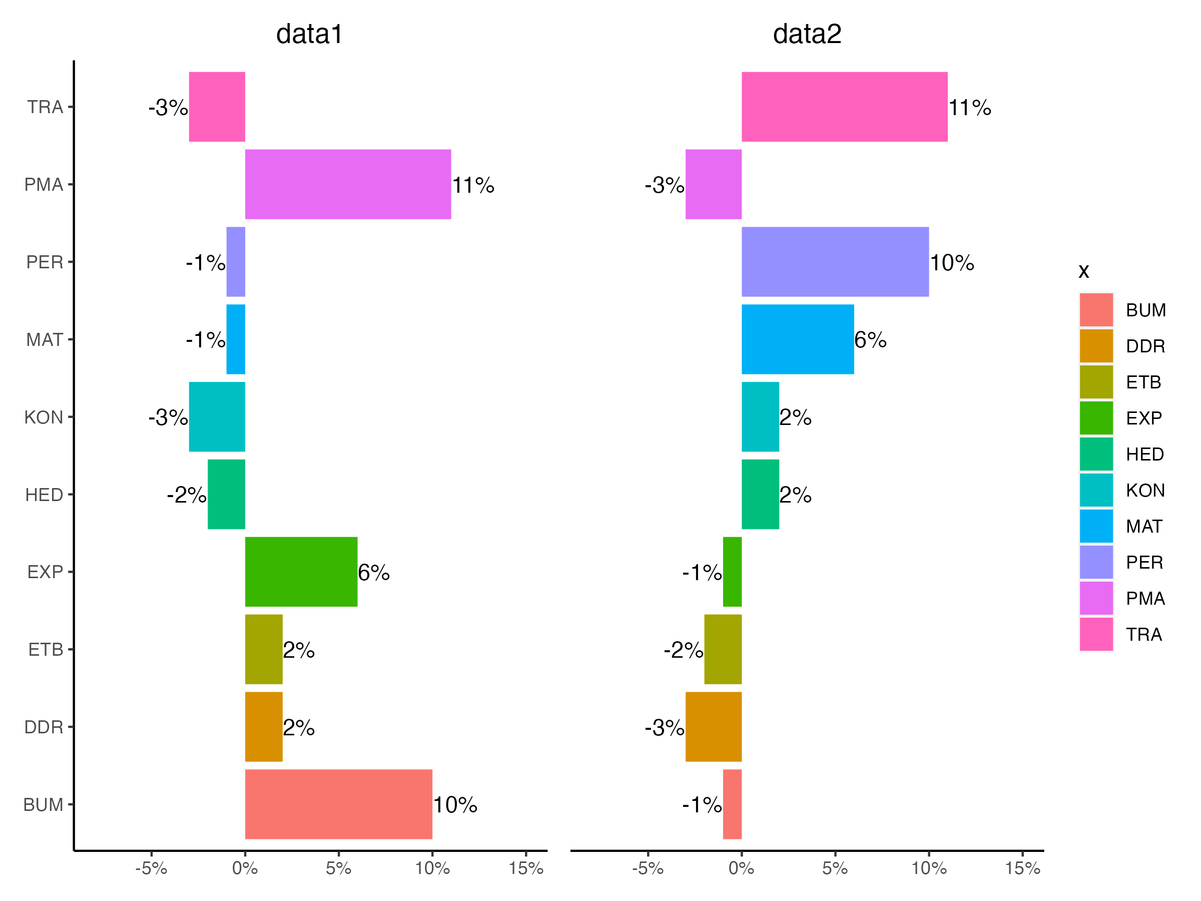
| 14:39, 15 December 2022 | Geom bar1.png (file) |  |
85 KB | Brb | <pre> library(ggplot2) library(scales) library(patchwork) dtf <- data.frame(x = c("ETB", "PMA", "PER", "KON", "TRA", "DDR", "BUM", "MAT", "HED", "EXP"), y = c(.02, .11, -.01, -.03, -.03, .02, .1, -.01, -.02, 0.06)) set.seed(1) dtf2 <- data.frame(x = dtf[, 1], y = sample(dtf[, 2])) g1 <- ggplot(dtf, aes(x, y)) + geom_bar(stat = "identity", aes(fill = x)) + geom_text(aes(label = paste0(y * 100, "%"), hjust = ifelse(y >= 0,... | 1 |
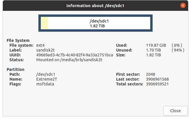
| 18:00, 5 December 2022 | GpartedinfoSanDisk.png (file) |  |
46 KB | Brb | 1 | |
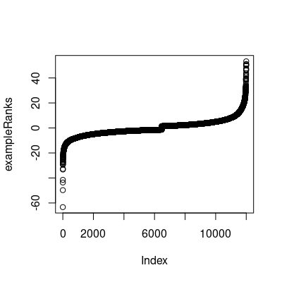
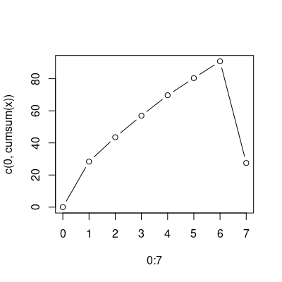
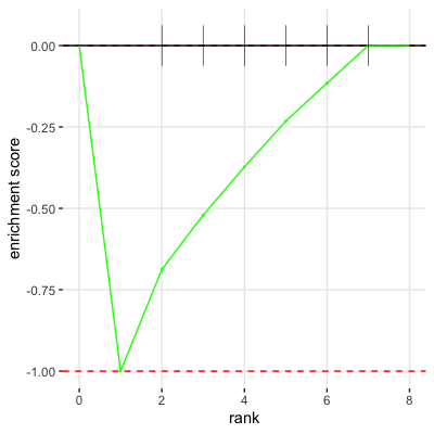
| 15:55, 29 October 2022 | ExampleRanks.png (file) |  |
6 KB | Brb | <pre> plot(exampleRanks) </pre> | 1 |
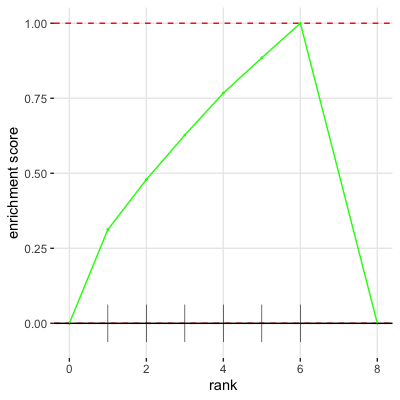
| 15:39, 29 October 2022 | FgseaPlotSmallm.png (file) |  |
7 KB | Brb | 1 | |
| 15:15, 27 October 2022 | DHdialog2.png (file) |  |
6 KB | Brb | 1 | |
| 15:15, 27 October 2022 | DHdialog1.png (file) |  |
21 KB | Brb | 1 | |
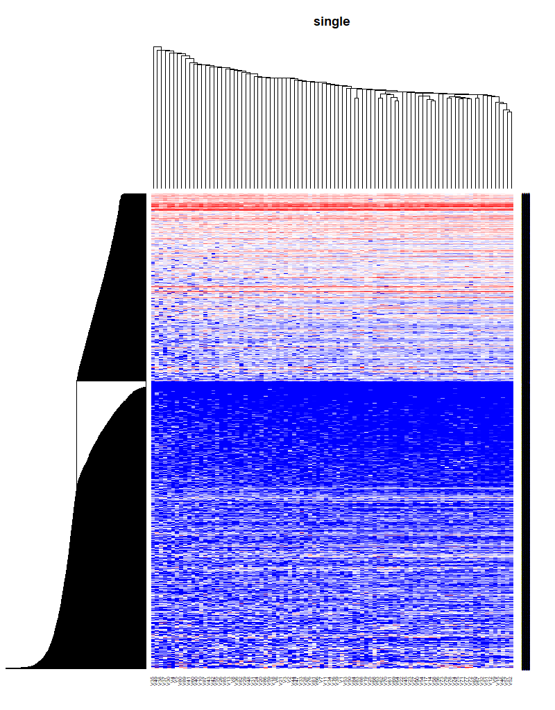
| 09:46, 27 October 2022 | HC single.png (file) |  |
133 KB | Brb | 1 | |
| 10:48, 20 October 2022 | 1NN better NC.png (file) |  |
18 KB | Brb | 1 | |
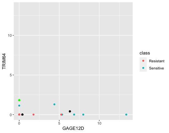
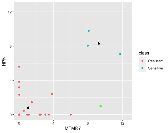
| 17:26, 19 October 2022 | NC better kNN.png (file) |  |
19 KB | Brb | The green color is a new observation (Sensitive). By using the kNN method, it will be assigned to Resistant b/c it is closer to the Resistant group. However, using the NC, the distance of it to the Resistant group centroid is 8.42 which is larger than the distance of it to the Sensitive groups centroid 7.31. So NC classified it to Sensitive. Color annotation: green=LOO obs, black=centroid in each class. | 1 |
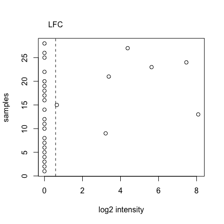
| 11:03, 12 October 2022 | Foldchangefilter.png (file) |  |
22 KB | Brb | <pre> LFC <- log2(1.5) x <- c(0, 0, 0, 0, 0, 0, 0, 0, 3.22, 0, 0, 0, 8.09, 0, 0.65, 0, 0, 0, 0, 0, 3.38, 0, 5.63, 7.46, 0, 0, 4.38, 0) plot(x, y = 1:28, xlab="log2 intensity", ylab="samples") abline(v=LFC, lty="dashed") axis(side=3,at=LFC, labels="LFC", tick=FALSE, line=0) </pre> | 1 |
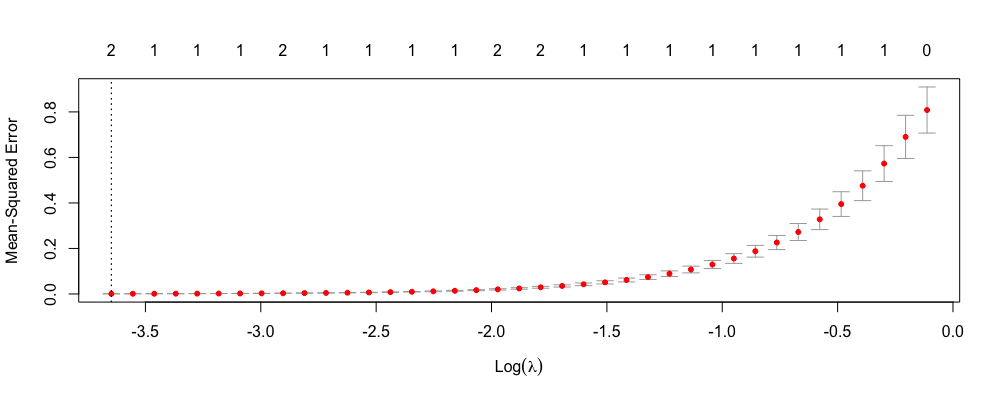
| 16:39, 11 October 2022 | Cvglmnetplot.png (file) |  |
34 KB | Brb | <pre> n <- 100 set.seed(1) x1 <- rnorm(n) e <- rnorm(n)*.01 y <- x1 + e x4 <- x fit <- cv.glmnet(x=cbind(x1, x4, matrix(rnorm(n*10), nr=n)), y=y) plot (fit) </pre> | 1 |
| 14:12, 6 October 2022 | Greedypairs.png (file) |  |
29 KB | Brb | 1 | |
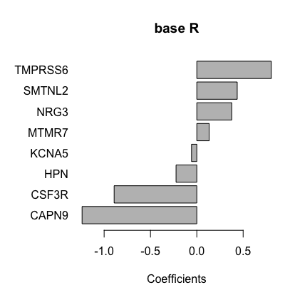
| 11:11, 6 October 2022 | Barplot base.png (file) |  |
20 KB | Brb | 2 | |
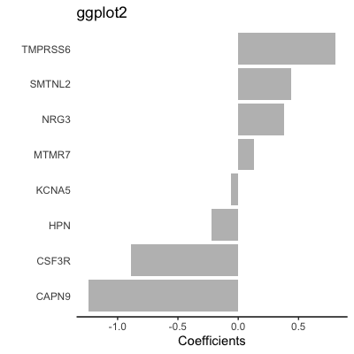
| 11:06, 6 October 2022 | Barplot ggplot2.png (file) |  |
16 KB | Brb | 1 | |
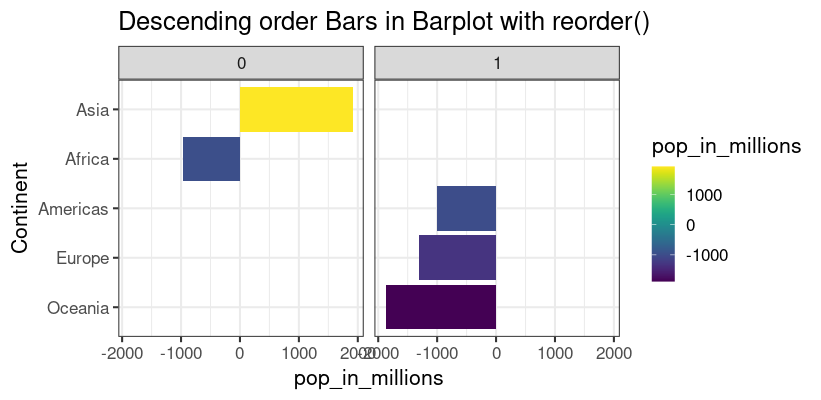
| 11:50, 30 August 2022 | Geomcolviridis.png (file) |  |
26 KB | Brb | Modify the example from https://datavizpyr.com/re-ordering-bars-in-barplot-in-r/ to allow filled colors and facet. <pre> library(tidyverse) library(gapminder) library(viridis) theme_set(theme_bw(base_size=16)) pop_df <- gapminder %>% filter(year==2007)%>% group_by(continent) %>% summarize(pop_in_millions=sum(pop)/1e06) pop_df2 <- tibble(class=rbinom(nrow(pop_df), 1, .5), pop_df) pop_df2 <- pop_df2 |> mutate(pop_in_millions = pop_in_millions-1900) pop_df2 %>% ggplot(aes... | 1 |
| 10:31, 30 August 2022 | ViridisDefault.png (file) |  |
2 KB | Brb | <pre> library(viridis) n = 200 image( 1:n, 1, as.matrix(1:n), col = viridis(n, option = "D"), xlab = "viridis n", ylab = "", xaxt = "n", yaxt = "n", bty = "n" ) </pre> | 1 |
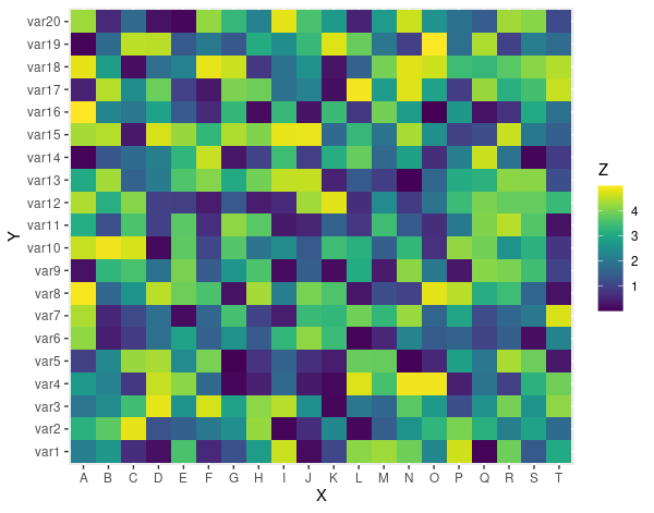
| 10:08, 30 August 2022 | ScaleFillViridisDiscrete.png (file) |  |
22 KB | Brb | See https://r-graph-gallery.com/79-levelplot-with-ggplot2.html <pre> library(ggplot2) # library(hrbrthemes) # Dummy data x <- LETTERS[1:20] y <- paste0("var", seq(1,20)) data <- expand.grid(X=x, Y=y) data$Z <- runif(400, 0, 5) library(viridis) ggplot(data, aes(X, Y, fill= Z)) + geom_tile() + scale_fill_viridis(discrete=FALSE) </pre> | 1 |
| 14:19, 29 August 2022 | Rbiomirgs barall.png (file) |  |
35 KB | Brb | 1 | |
| 14:17, 29 August 2022 | Rbiomirgs bar.png (file) |  |
92 KB | Brb | 1 | |
| 14:17, 29 August 2022 | Rbiomirgs volcano.png (file) |  |
66 KB | Brb | 1 | |
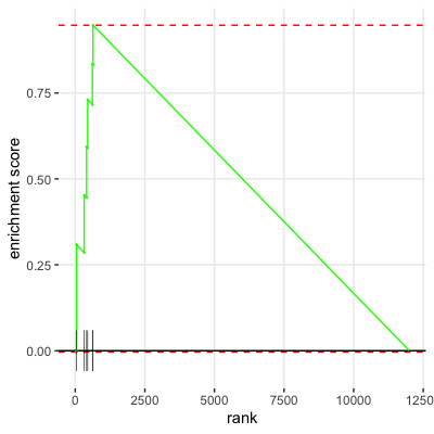
| 07:08, 27 August 2022 | FgseaPlotTop.png (file) | 15 KB | Brb | 1 | ||
| 06:34, 27 August 2022 | FgseaPlotSmall2.png (file) |  |
23 KB | Brb | 1 | |
| 06:34, 27 August 2022 | FgseaPlotSmall.png (file) |  |
24 KB | Brb | 1 | |
| 06:33, 27 August 2022 | FgseaPlot.png (file) |  |
23 KB | Brb | 1 | |
| 15:02, 23 August 2022 | ComplexHeatmap1.png (file) |  |
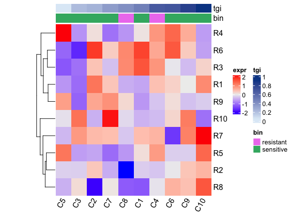
29 KB | Brb | <pre> library(ComplexHeatmap) set.seed(123) ng <- 10; n <- 10 mat = matrix(rnorm(ng * n), n) rownames(mat) = paste0("R", 1:ng) colnames(mat) = paste0("C", 1:n) bin <- sample(c("resistant", "sensitive"), n, replace = TRUE) tgi <- runif(n) # sort the columns by tgi ord <- order(tgi) col_fun = circlize::colorRamp2(range(tgi), c("#DEEBF7", "#084594")) column_ha = HeatmapAnnotation(tgi = tgi[ord], bin = bin[ord], col = list(tgi = col_fun,... | 1 |
| 14:19, 22 August 2022 | Doubledip.png (file) |  |
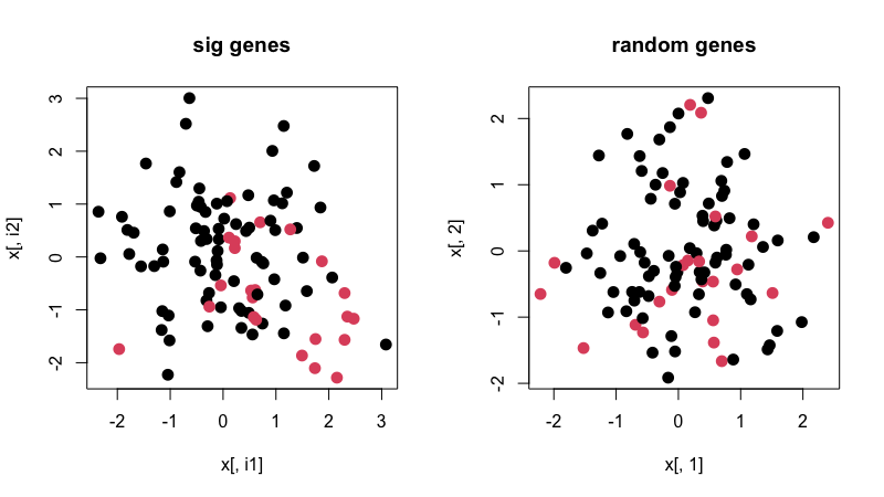
57 KB | Brb | <pre> ng <- 1000 # number of genes ns <- 100 # number of samples k <- 2 # number of groups alpha <- .001 # cutoff of selecting sig genes set.seed(1) x = matrix(rnorm(ng * ns), nr= ns) # samples x features hc = hclust(dist(x)) plot(hc) grp = cutree(hc, k=k) # vector of group membership ex <- t(x) r1 <- genefilter::rowttests(ex, factor(grp)) sum(r1$p.value < alpha) # 2 hist(r1$p.value) i <- which(r1$p.value < alpha) i1 <- i[1] ; i2 <- i[2] plot(x[, i1], x[, i2], col = grp, pch= 16, cex=1... | 1 |
| 10:21, 10 August 2022 | Ruspini.png (file) |  |
81 KB | Brb | library(cluster) # ruspini is 75 x 2 data(ruspini) hc <- hclust(dist(ruspini), "ave"); plot(hc) # si <- silhouette(groups, dist(ruspini)) # plot(si, main = paste("k = ", 4)) op <- par(mfrow= c(3,2), oma= c(0,0, 3, 0), mgp= c(1.6,.8,0), mar= .1+c(4,2,2,2)) plot(hc) for(k in 2:6) { groups<- cutree(hc, k=k) si <- silhouette(groups, dist(ruspini)) plot(si, main = paste("k = ", k)) } par(op) | 1 |
| 19:55, 23 June 2022 | Tidyheatmap.png (file) |  |
50 KB | Brb | 1 | |
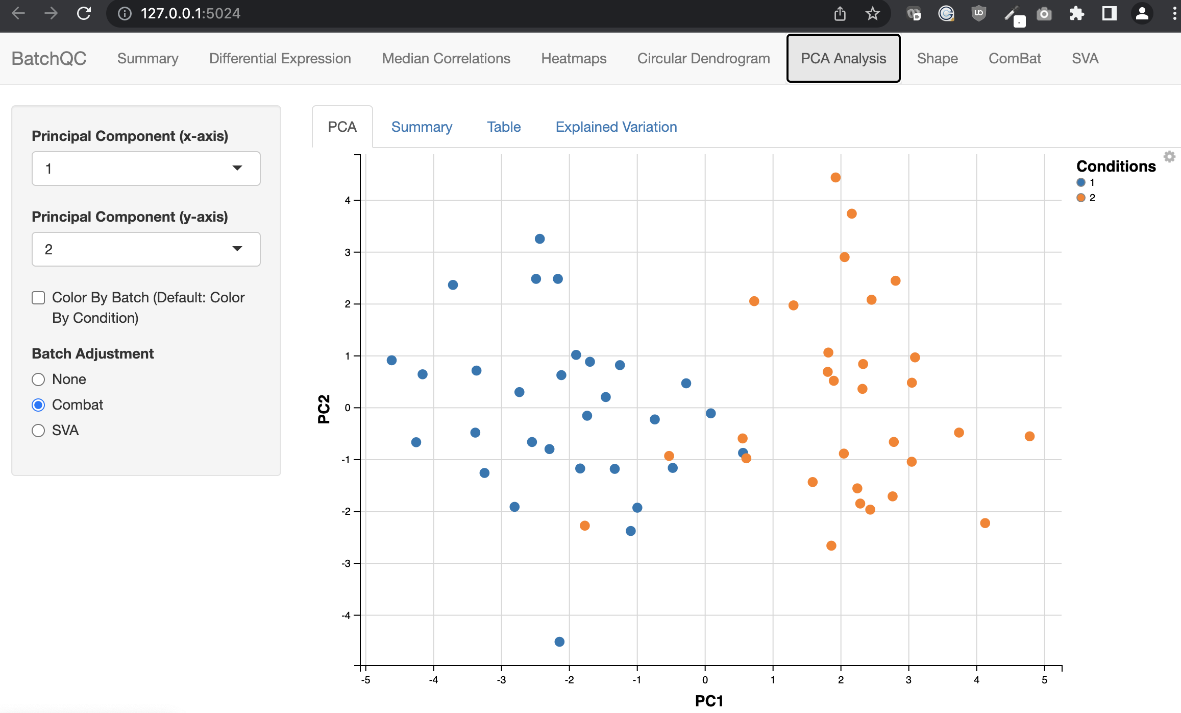
| 15:22, 21 June 2022 | BatchqcPCA.png (file) |  |
320 KB | Brb | 1 | |
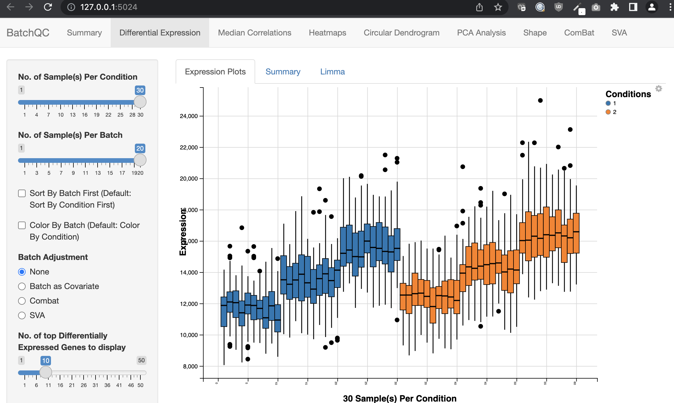
| 15:22, 21 June 2022 | BatchqcDE.png (file) |  |
391 KB | Brb | 1 | |
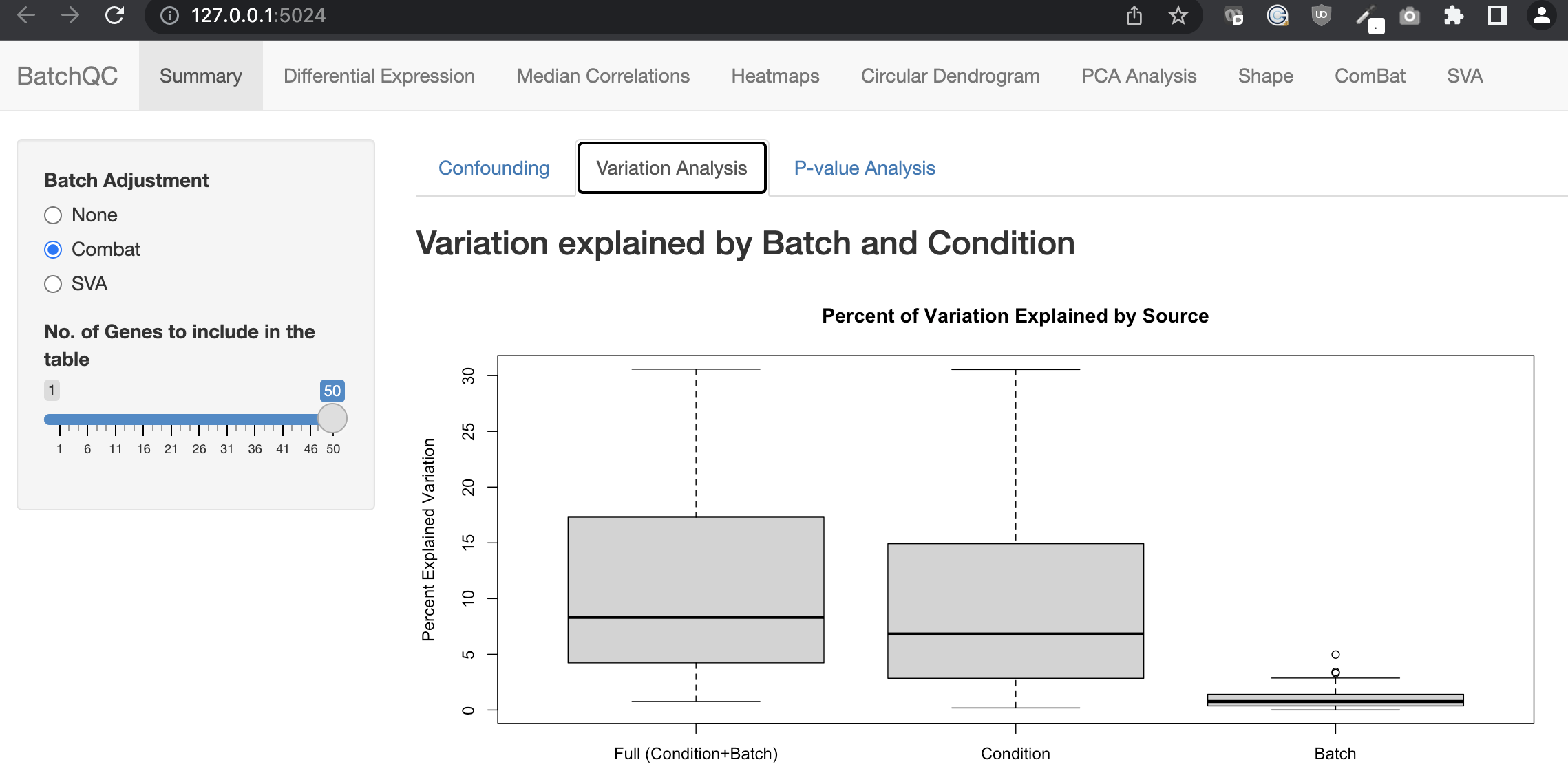
| 15:21, 21 June 2022 | BatchqcVariation.png (file) |  |
267 KB | Brb | 1 | |
| 15:20, 21 June 2022 | BatchqcSummary.png (file) |  |
307 KB | Brb | 1 | |
| 18:02, 4 June 2022 | Heatmap rdylbu.png (file) |  |
30 KB | Brb | 1 | |
| 10:06, 27 May 2022 | Inter gg2.png (file) |  |
40 KB | Brb | 1 | |
| 09:51, 27 May 2022 | Inter gg.png (file) |  |
21 KB | Brb | 1 | |
| 09:51, 27 May 2022 | Inter base.png (file) |  |
15 KB | Brb | 1 | |
| 09:16, 27 May 2022 | Inter base.svg (file) |  |
35 KB | Brb | 2 | |
| 10:08, 26 May 2022 | LogisticFail.svg (file) |  |
25 KB | Brb | > set.seed(1234); n <- 16; mu=3; x <- c(rnorm(n), rnorm(n, mu)); y <- rep(0:1, each=n) > summary(glm(y ~ x, family = binomial)); plot(x, y) | 1 |
| 12:56, 10 May 2022 | ColorRampBlueRed.png (file) |  |
4 KB | Brb | 1 | |
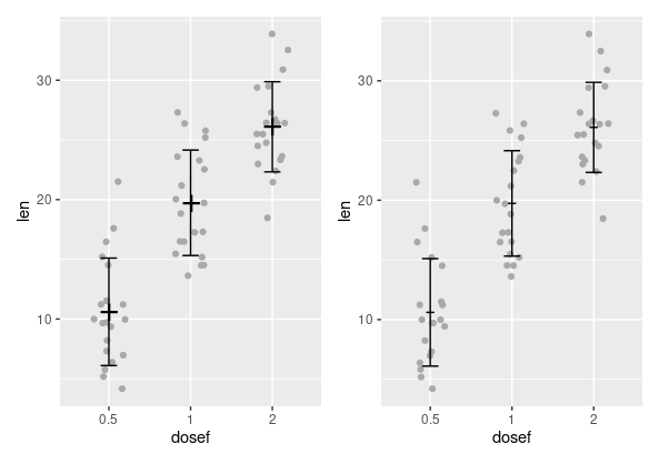
| 19:39, 24 March 2022 | Rerrorbars.png (file) |  |
10 KB | Brb | <pre> library(ggplot2) df <- ToothGrowth df$dosef <- as.factor(df$dose) library(dplyr) df.summary <- df %>% group_by(dosef) %>% summarise( sd = sd(len, na.rm = TRUE), len = mean(len) ) df.summary p1 <- ggplot(df, aes(dosef, len)) + geom_jitter(position = position_jitter(0.2, seed=1), color = "darkgray") + geom_point(aes(x=dosef, y=len), shape="+", size=8, data=df.summary) + geom_errorbar(aes(ymin = len-sd, ymax = len+sd), width=.2, data = df.summary) df.summary$dose <... | 1 |
| 19:37, 24 March 2022 | Rerrorbar.svg (file) |  |
75 KB | Brb | <pre> library(ggplot2) df <- ToothGrowth df$dosef <- as.factor(df$dose) library(dplyr) df.summary <- df %>% group_by(dosef) %>% summarise( sd = sd(len, na.rm = TRUE), len = mean(len) ) df.summary p1 <- ggplot(df, aes(dosef, len)) + geom_jitter(position = position_jitter(0.2, seed=1), color = "darkgray") + geom_point(aes(x=dosef, y=len), shape="+", size=8, data=df.summary) + geom_errorbar(aes(ymin = len-sd, ymax = len+sd), width=.2, data = df.summary) df.summary$dose <... | 1 |