GEO
Gene Expression Omnibus (GEO) website is located at http://www.ncbi.nlm.nih.gov/geo/. GEO is a public functional genomics data repository supporting MIAME-compliant data submissions. Array- and sequence-based data are accepted. Tools are provided to help users query and download experiments and curated gene expression profiles.
Browse Content
Repository Browser/Summary
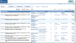
Click on 'Browse Content' > 'Repository Browser' to go to the summary page. It has 4 tabs.
Series/Series Type
Expression profiling by array	40,319
Expression profiling by genome tiling array	639
Expression profiling by high throughput sequencing	4,772
Expression profiling by SAGE	242
Expression profiling by MPSS	20
Expression profiling by RT-PCR	329
Expression profiling by SNP array	13
Genome variation profiling by array	596
Genome variation profiling by genome tiling array	1,068
Genome variation profiling by high throughput sequencing	63
Genome variation profiling by SNP array	826
Genome binding/occupancy profiling by array	174
Genome binding/occupancy profiling by genome tiling array	2,114
Genome binding/occupancy profiling by high throughput sequencing	3,940
Genome binding/occupancy profiling by SNP array	12
Methylation profiling by array	556
Methylation profiling by genome tiling array	718
Methylation profiling by high throughput sequencing	764
Methylation profiling by SNP array	9
Protein profiling by protein array	167
Protein profiling by Mass Spec	6
SNP genotyping by SNP array	514
Other	1,147
Non-coding RNA profiling by array	2,166
Non-coding RNA profiling by genome tiling array	104
Non-coding RNA profiling by high throughput sequencing	1,478
Third-party reanalysis	135
The R code to query this information is
library(GEOmetadb)
sfile = 'GEOmetadb.sqlite'
if(!file.exists(sfile)) {
  sfile = getSQLiteFile()
}

library(dplyr)
gmdb = src_sqlite(sfile)
# List available tables in the database
src_tbls(gmdb)

tgse = tbl(gmdb,'gse')
tgsm = tbl(gmdb,'gsm')
tgpl = tbl(gmdb,'gpl')

library(tidyr)
gse_type = select(tgse,gse,type) %>%
  transform(type = strsplit(type,';\\t')) %>%
  unnest(type)
type_count = select(gse_type,type) %>%
  group_by(type) %>%
  summarize(count=n()) %>%
  arrange(desc(count))
pander(type_count,justify=c('left','right'))
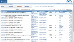
Platform/Technology
Technology	Count
in situ oligonucleotide	5,657
spotted oligonucleotide	2,852
spotted DNA/cDNA	2,869
antibody	24
MS	17
SAGE NlaIII	67
SAGE Sau3A	4
SAGE RsaI	1
SARST	2
MPSS	18
RT-PCR	277
other	174
oligonucleotide beads	227
mixed spotted oligonucleotide/cDNA	16
spotted peptide or protein	110
high-throughput sequencing	2,073
Some examples
- hgu-133a GPL96 22283 rows
- hgu-133b GPL97 22645 rows
- hgu-133 plus 2.0 GPL570 54675 rows
- hgu-133a 2.0 GPL571 22277 rows
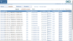
Samples/Samples Type
Sample type	Count
RNA	1,017,959
genomic	244,511
protein	12,860
SAGE	1,763
mixed	3,976
other	7,509
SARST	9
MPSS	207
SRA	135,247
Organism
A partial list:
Organism	Series	Platforms	Samples
Homo sapiens	22,477	4,590	792,844
Mus musculus	15,758	1,959	240,935
Rattus norvegicus	2,358	475	68,583
Saccharomyces cerevisiae	1,790	550	37,435
Arabidopsis thaliana	2,416	331	30,709
Drosophila melanogaster	2,422	317	23,601
Sus scrofa	405	107	9,809
Caenorhabditis elegans	1,154	183	8,898
Zea mays	265	91	8,667
Bos taurus	462	147	7,780
Oryza sativa	493	173	5,616
Glycine max	179	41	5,863
Gallus gallus	375	105	5,509
Escherichia coli	508	127	5,056
Macaca mulatta	245	40	4,504
Xenopus laevis	111	25	1,054
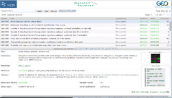
Series, Samples, Platforms, DataSets
R packages
GEOmetadb
- http://gbnci.abcc.ncifcrf.gov/geo/ Meltzerlab GEO Microarray Tool
- https://nsaunders.wordpress.com/2010/08/30/geo-database-curation-lagging-behind-submission/
- http://rpubs.com/seandavi/GEOMetadbSurvey2014 dplyr and the GEOmetadb package for mining NCBI GEO metadata]
GEOsubmission
Converts a microarray dataset and the corresponding sample information into a SOFT file to be used for GEO submission.
GEOquery
Retrieve GSE
- http://bioconductor.org/packages/release/bioc/vignettes/GEOquery/inst/doc/GEOquery.html. It seems the output class of getGEO() depends on the GSEMatrix argument. Method 1. Retrieve series matrix (GSE9782-GPL96_series_matrix.txt.gz is 21MB, GSE9782-GPL97_series_matrix.txt.gz is 21MB). The phenotype is located at the header; grep "characteristics". This is fast and should be considered first.
- S4 methods: exprs(), pData(), fData(), et al; see methods(class = "ExpressionSet").
library(GEOquery)

# Series matrix. Pro: get gene expression, pheno data, feature data, much small object
gse <- getGEO("GSE9782") # By default, GSEMatrix = TRUE & getGPL = TRUE
class(gse)
# [1] "list"
head(Meta(gse))
# Error in (function (classes, fdef, mtable)  :
#  unable to find an inherited method for function ‘Meta’ for signature ‘"list"’
Meta(gse[[1]])
# Error in (function (classes, fdef, mtable)  :
#   unable to find an inherited method for function ‘Meta’ for signature ‘"ExpressionSet"’
names(GPLList(gse))
# Error in (function (classes, fdef, mtable)  :
#  unable to find an inherited method for function ‘GPLList’ for signature ‘"list"’

show(gse)  # length of 2, GPL96 & GPL97

# Get the expression matrix
mat1 <- exprs(gse[[1]])
dim(mat1) # 22283 x 264
mat1[1:2, 1:5]
          GSM246523 GSM246524 GSM246525 GSM246526 GSM246527
1007_s_at   235.523  498.2220  309.2070   307.569   37.3808
1053_at      41.447   69.0219   69.3994    36.931   43.5677

mat2 <- exprs(gse[[2]])
dim(mat2) # 22645 x 264

library(magrittr)
intersect(rownames(mat1), rownames(mat2)) %>% length()
# [1] 168

# Get the phenotype information
dim(pData(gse[[1]]))
# [1] 264  53
pData(gse[[1]])[1:2, 1:3]
#               title geo_accession                status
# GSM246523 MPM002090     GSM246523 Public on Dec 06 2007
# GSM246524 MPM002091     GSM246524 Public on Dec 06 2007

# the expression matrix is an ExpressionSet object, ready for limma
class(gse[[1]])
# [1] "ExpressionSet"
# attr(,"package")
# [1] "Biobase"

# However, the GSM from GPL96 and GPL97 are independent
pData(gse[[2]])[1:5, 2]
# [1] "GSM246787" "GSM246788" "GSM246789" "GSM246790" "GSM246791"
pData(gse[[1]])[1:5, 2]
# [1] "GSM246523" "GSM246524" "GSM246525" "GSM246526" "GSM246527"
intersect(pData(gse[[1]])[, 2], pData(gse[[2]])[, 2])
# character(0)

# We can match samples from GPL96 and GPL97 via 'title' (1st column)
intersect(pData(gse[[1]])[, "title"], pData(gse[[2]])[, "title"]) %>% length()
# [1] 264

# Access feature data
fData(gse[[1]]) %>% colnames()
#  [1] "ID"                               "GB_ACC"
#  [3] "SPOT_ID"                          "Species Scientific Name"
#  [5] "Annotation Date"                  "Sequence Type"
#  [7] "Sequence Source"                  "Target Description"
#  [9] "Representative Public ID"         "Gene Title"
# [11] "Gene Symbol"                      "ENTREZ_GENE_ID"
# [13] "RefSeq Transcript ID"             "Gene Ontology Biological Process"
# [15] "Gene Ontology Cellular Component" "Gene Ontology Molecular Function"
fData(gse[[1]]) %>% dim()
# [1] 22283    16
fData(gse[[1]])[1:5, c("ID", "Gene Symbol", "ENTREZ_GENE_ID")]
#                  ID      Gene Symbol    ENTREZ_GENE_ID
# 1007_s_at 1007_s_at DDR1 /// MIR4640 780 /// 100616237
# 1053_at     1053_at             RFC2              5982
# 117_at       117_at            HSPA6              3310
# 121_at       121_at             PAX8              7849
# 1255_g_at 1255_g_at           GUCA1A              2978
Method 2. Retrieve soft data (GSE9782_family.soft.gz is 89 MB). Like series matrix, it contains gene expression, phenotype data but this file size is huge (why?) and the phenotype is not located at the header. Note I is not clear how to use get the phenotype data when we use getGEO(, GSEMatrix=F) approach.# Obtain the soft format file. Pro: meta data; e.g. GPLlist(), GSMList() gse2 <- getGEO("GSE9782",GSEMatrix=F) class(gse2) # [1] "GSE" # attr(,"package") # [1] "GEOquery" head(Meta(gse2)) # $contact_address # [1] "35 Landsdowne Stree" # $contact_city # [1] "Cambridge" # ... Meta(gse2)$type # [1] "Expression profiling by array" Meta(gse2)$platform_id # [1] "GPL96" "GPL97" print(object.size(gse), units = "auto") # 65.2 Mb print(object.size(gse2), units = "auto") # 974.6 Mb names(GSMList(gse2)) %>% head() # [1] "GSM246523" "GSM246524" "GSM246525" "GSM246526" "GSM246527" "GSM246528" names(GSMList(gse2)) %>% length() # [1] 528 names(GPLList(gse2)) # [1] "GPL96" "GPL97" length(GSMList(gse2)) # [1] 528 class(GSMList(gse2)[[1]]) # [1] "GSM" # attr(,"package") [1] "GEOquery" - http://watson.nci.nih.gov/~sdavis/tutorials/CSHL2010/publicRepos.html
- Accessing Public Data using R and Bioconductor
- http://www2.warwick.ac.uk/fac/sci/moac/people/students/peter_cock/r/geo
- https://www.biostars.org/p/4896/, https://www.biostars.org/p/111791/
- Creating Annotated Data Frames from GEO with the GEOquery package
Question: how many GSE series from GPL198? How many samples in each of these series?
Retrieve GPL and subset expression
We can retrieve the annotation data for a specific GPL.
gpl96 <- getGEO("GPL96")
Meta(gpl96)

colnames(Table(gpl96))
#  [1] "ID"                               "GB_ACC"
#  [3] "SPOT_ID"                          "Species Scientific Name"
#  [5] "Annotation Date"                  "Sequence Type"
#  [7] "Sequence Source"                  "Target Description"
#  [9] "Representative Public ID"         "Gene Title"
# [11] "Gene Symbol"                      "ENTREZ_GENE_ID"
# [13] "RefSeq Transcript ID"             "Gene Ontology Biological Process"
# [15] "Gene Ontology Cellular Component" "Gene Ontology Molecular Function"

Table(gpl96)[1:5, c("ID", "Gene Symbol", "ENTREZ_GENE_ID")]
#          ID      Gene Symbol    ENTREZ_GENE_ID
# 1 1007_s_at DDR1 /// MIR4640 780 /// 100616237
# 2   1053_at             RFC2              5982
# 3    117_at            HSPA6              3310
# 4    121_at             PAX8              7849
# 5 1255_g_at           GUCA1A              2978

dim(Table(gpl96))
# [1] 22283    16
gpl97 <- getGEO("GPL97")
dim(Table(gpl97))
# [1] 22645    16
We can further to subset the genes by getting the gene expression data for all the probes with a gene symbol; see eg here.
SRAdb
SRA website is located at http://www.ncbi.nlm.nih.gov/Traces/sra/sra.cgi
rentrez
Provides an R interface to the NCBI's 'EUtils' API, allowing users to search databases like 'GenBank' <https://www.ncbi.nlm.nih.gov/genbank/> and 'PubMed' <https://www.ncbi.nlm.nih.gov/pubmed/>, process the results of those searches and pull data into their R sessions.
- https://cran.r-project.org/web/packages/rentrez/vignettes/rentrez_tutorial.html
- https://www.r-bloggers.com/a-rentrez-paper-and-how-to-use-the-ncbis-new-api-keys/
BART (bioinformatics array research tool): R shiny application for microarray analysis
Some cases
GSE22631
Agilent-014879 Whole Rat Genome Microarray 4x44K G4131F. 12 samples.
Soft format
27MB after decompression. It contains gene annotation for that platform, gene expression and sample information. The format is however not a matrix format. For example, after the gene annotation, the rest of files are separated by samples with 1 column (VALUE) representing gene expression.
See https://gist.github.com/arraytools/9a6e954ef423d6634695#file-gse22631_family-soft.
Series matrix
These files are suitable for loading in MS-Excel.
6MB after decompression. It contains gene expression (no gene annotation) and sample information.
The sample information is on the header. But we need to transpose that in order to get the normal form where each row is a sample and each column is a variable.
See https://gist.github.com/arraytools/9a6e954ef423d6634695#file-gse22631_series_matrix-txt.
Experiment descriptor (ArrayTools)
See https://gist.github.com/arraytools/9a6e954ef423d6634695#file-experiment-descriptors.
GDS507
This is a data used by GEOquery package. 17 samples. HG-U133B platform.
There is a related GSE number (GSE781) for this GDS data. However, GSE781 is a larger dataset and contains two platforms (HG-U133A and HG-U133B). It has 34 samples.
The raw cel files are available too.
GSE30786
This is actually an RNA-Seq data. There are 4 samples with 2 conditions. See
GSE20986
HGU133 plus 2. 12 arrays.
The CEL files were processed with the BioConductor gcrma function.
GSE68465
HGU133A.
The CEL files were processed with MAS5.
GSE6532 (HG-U133A + HG-U133B)
Breast cancer data used by Tian 2014. Processed data in RData format is available. RMA normalized signal intensity is provided in series matrix.
# Consider the 1st sample gsm65316
x <- read.delim(url("https://www.ncbi.nlm.nih.gov/geo/query/acc.cgi?view=data&acc=GSM65316&id=34328&db=GeoDb_blob01"), skip=22, header = F)

summary(x[, 2])
#   Min. 1st Qu.  Median    Mean 3rd Qu.    Max.    NA's
#  3.364   5.760   6.970   7.070   8.242  14.206       7
summary(2^x[, 2])
#   Min. 1st Qu.  Median    Mean 3rd Qu.    Max.    NA's
#   10.3    54.2   125.4   351.5   302.7 18896.8       7
GSE9782 (HG-U133A + HG-U133B)
Multiple myeloma data used by Mulligan 2006. MAS5 signal intensity can be obtained from series matrix.
GEO2R
RNA-Seq
- Search, Download, and Visualize Human RNA-Seq Gene Expression Data in NCBI’s Gene Expression Omnibus (GEO) & a comment from M Love
- *NCBI-generated RNA-seq count data (Beta)
- HISAT2
- Subread featureCounts
- Using the raw counts as input, GEO then computes FPKM(RPKM) and TPM normalized values.
- The pipeline continues to process new RNA-seq data as it is submitted to SRA, with a turnaround time of approximately one week
- rnaseq counts and Homo sapiens 22121 results as of 6/7/2023
GEOexplorer
GEOexplorer – a webserver for gene expression analysis and visualisation
Tips
Gene symbol aliases
For example EZHIP has an alias CXorf67. CXorf67 can be found in GPL570 but not GPL96 or GPL97.
R> library(GEOquery)
R> gpl570 <- getGEO("GPL570")
R> grep("EZHIP", Table(gpl570)$"Gene Symbol")
integer(0)
R> grep("CXorf67", Table(gpl570)$"Gene Symbol")
[1] 2298

R> gpl96 <- getGEO("GPL96")
R> grep("CXorf67", Table(gpl96)$"Gene Symbol")
integer(0)
R> gpl97 <- getGEO("GPL97")
R> grep("CXorf67", Table(gpl97)$"Gene Symbol")
integer(0)
Using the Bioconductor annotation package,
> library(hgu133plus2.db)

> k <- keys(hgu133plus2.db, keytype="PROBEID")
> k2 <- select(hgu133plus2.db, keys=k, columns=c("SYMBOL","GENENAME"), keytype="PROBEID")
'select()' returned 1:many mapping between keys and columns
> dim(k2)
[1] 58363     3
> k2[1:3, ]
    PROBEID  SYMBOL                                    GENENAME
1 1007_s_at    DDR1 discoidin domain receptor tyrosine kinase 1
2 1007_s_at MIR4640                               microRNA 4640
3   1053_at    RFC2              replication factor C subunit 2
> select(hgu133a.db, keys=k, columns=c("SYMBOL","GENENAME"), keytype="PROBEID")
> grep("CXorf67", k2$SYMBOL)
integer(0)
> grep("EZHIP", k2$SYMBOL)
[1] 2400
> k2[2400, ]
          PROBEID SYMBOL               GENENAME
2400 1555396_s_at  EZHIP EZH inhibitory protein
Search articles in PubMed
- Find: Research in context. A gene-expression profiling score for outcome prediction disease in patients with follicular lymphoma: a retrospective analysis on three international cohorts.
Find GEO dataset
- https://wiki.bits.vib.be/index.php/Find_GEO_datasets
- https://academic.oup.com/nar/article/33/suppl_1/D562/2505234#42612985
- https://guides.lib.berkeley.edu/c.php?g=403317&p=6553361
- https://www.r-bloggers.com/samples-per-seriesdataset-in-the-ncbi-geo-database/
Search by SRRxxxxxx
Search the SRA website; for example SRR902884.
Explore GEO/SRA
Download reads from repositories like NCBI SRA
A Step‐by‐Step Guide to Submitting RNA‐Seq Data to NCBI
https://currentprotocols.onlinelibrary.wiley.com/doi/pdf/10.1002/cpbi.67
Other public data repositories
ArrayExpress
https://www.ebi.ac.uk/arrayexpress/
the Cancer Genome Atlas / TCGA
- http://cancergenome.nih.gov/
- https://www.cbioportal.org/
- TCGA2STAT R package
- Genome → cBioPortal and TCGA
dbGaP
https://www.ncbi.nlm.nih.gov/gap/
International Cancer Genome Consortium / ICGC
www.icgc.org
Cell line growth response and sequencing data
NCI60, CCLE, GDSC-Sanger (Genomics of Drug Sensitivity in Cancer), https://discover.nci.nih.gov/cellminercdb/
Drug response
- Google: bioconductor drug response data
- Clinical drug response can be predicted using baseline gene expression levels and in vitro drug sensitivity in cell lines breast cancer (GSE 6434) & myeloma (GSE9782) & NSCLC cancer (GSE 33072), 2014
- BloodCancerMultiOmics2017 "Drug-perturbation-based stratification of blood cancer"
- rcellminerData: Molecular Profiles and Drug Response for the NCI-60 Cell Lines
- Predict drug sensitivity of cancer cells with pathway activity inference 2019
- Assessment of modelling strategies for drug response prediction in cell lines and xenografts 2020
- oncoPredict: an R package for predicting in vivo or cancer patient drug response and biomarkers from cell line screening data Briefings in Bioinformatics 2021, CRAN.
- synergyfinder Calculate and Visualize Synergy Scores for Drug Combinations. paper 2022
- Predicting tumor drug sensitivity with multi-omics data


