PCA
Principal component analysis
What is PCA
- https://en.wikipedia.org/wiki/Principal_component_analysis
- StatQuest: Principal Component Analysis (PCA), Step-by-Step (video)
- StatQuest: PCA in R
- Using R for Multivariate Analysis
- How exactly does PCA work? What PCA (with SVD) does is, it finds the best fit line for these data points which minimizes the distance between the data points and their projections on the best fit line.
- What Is Principal Component Analysis (PCA) and How It Is Used? PCA creates a visualization of data that minimizes residual variance in the least squares sense and maximizes the variance of the projection coordinates.
- Principal Component Analysis: a brief intro for biologists
Linear Algebra
Linear Algebra for Data Science with examples in R
R source code
> stats:::prcomp.default
function (x, retx = TRUE, center = TRUE, scale. = FALSE, tol = NULL,
    ...)
{
    x <- as.matrix(x)
    x <- scale(x, center = center, scale = scale.)
    cen <- attr(x, "scaled:center")
    sc <- attr(x, "scaled:scale")
    if (any(sc == 0))
        stop("cannot rescale a constant/zero column to unit variance")
    s <- svd(x, nu = 0)
    s$d <- s$d/sqrt(max(1, nrow(x) - 1))
    if (!is.null(tol)) {
        rank <- sum(s$d > (s$d[1L] * tol))
        if (rank < ncol(x)) {
            s$v <- s$v[, 1L:rank, drop = FALSE]
            s$d <- s$d[1L:rank]
        }
    }
    dimnames(s$v) <- list(colnames(x), paste0("PC", seq_len(ncol(s$v))))
    r <- list(sdev = s$d, rotation = s$v, center = if (is.null(cen)) FALSE else cen,
        scale = if (is.null(sc)) FALSE else sc)
    if (retx)
        r$x <- x %*% s$v
    class(r) <- "prcomp"
    r
}
<bytecode: 0x000000003296c7d8>
<environment: namespace:stats>
rank of a matrix
R example
Principal component analysis (PCA) in R including bi-plot.
R built-in plot
http://genomicsclass.github.io/book/pages/pca_svd.html
pc <- prcomp(x)
group <- as.numeric(tab$Tissue)
plot(pc$x[, 1], pc$x[, 2], col = group, main = "PCA", xlab = "PC1", ylab = "PC2")
The meaning of colors can be found by palette().
- black
- red
- green3
- blue
- cyan
- magenta
- yellow
- gray
palmerpenguins data
Theory with an example
Principal Component Analysis in R: prcomp vs princomp
Biplot
- Biplots are everywhere: where do they come from?
- ggbiplot. Principal Component Analysis in R Tutorial from datacamp.
- Exploring Multivariate Data with Principal Component Analysis (PCA) Biplot in R including the interpretation.
- Biplot of PCA in R (Examples) using both base R and factoextra package
- 5 PCA Visualizations You Must Try On Your Next Data Science Project including the interpretation of biplot.
factoextra
- https://cran.r-project.org/web/packages/factoextra/index.html
- Factoextra R Package: Easy Multivariate Data Analyses and Elegant Visualization
Properties
- Definition. If x is a random vector with mean [math]\displaystyle{ \mu }[/math] and covariance matrix [math]\displaystyle{ \Sigma }[/math], the the principal component transformation is
- [math]\displaystyle{ y = \Gamma ' (x - \mu), }[/math]
- Properties
- [math]\displaystyle{ E(y_i) =0, }[/math]
- [math]\displaystyle{ Var(y_i) =\lambda_i, }[/math]
- [math]\displaystyle{ Cov(y_i, y_j) =0, i \neq j, }[/math]
- [math]\displaystyle{ Var(y_1) \geq Var(y_2) \geq \cdots Var(y_p) \geq 0, }[/math]
- [math]\displaystyle{ \sum Var(y_i) = tr \Sigma, }[/math] total variation
- [math]\displaystyle{ \prod Var(y_i) = |\Sigma| }[/math].
- The sum of the first k eigenvalues divided by the sum of all the eigenvalues, [math]\displaystyle{ (\lambda_1 + \cdots + \lambda_k)/(\lambda_1 + \cdots + \lambda_p) }[/math], represents the proportion of total variation explained by the first k principal components.
- The principal component of a random vector are not scale-invariant. For example, given three variables, say weight in pounds, height in feet, and age in years, we may seek a principal component expressed say in ounces, inches, and decades. Two procedures see feasible:
- Multiple the data by 16, 12 and .1, respectively, and then carry out a PCA,
- Carry out a PCA and then multiply the elements of the relevant component by 16, 12 and .1.
- Number of principals?
- Include just enough components to explain say 90% of the total variations scree graph;
- Exclude those principal components whose eigenvalues are less than the average (Kaiser)
- Rotation/loadings matrix is orthogonal
x <- matrix(c(10,6,12,5,11,4,9,7,8,5,10,6,3,3,2.5,2,2,2.8,1.3,4,1,1,2,7), nr=4) x <- t(x) # 6 samples, 4 genes rownames(x) <- paste("mouse",1:6) colnames(x) <- paste("gene", 1:4) pr <- prcomp(x, scale = T) t(pr$rotation) %*% pr$rotation - diag(4) # PC1 PC2 PC3 PC4 # PC1 0.000000e+00 0.000000e+00 1.804112e-16 -2.081668e-17 # PC2 0.000000e+00 -1.110223e-16 1.387779e-16 -2.220446e-16 # PC3 1.804112e-16 1.387779e-16 -2.220446e-16 -5.551115e-17 # PC4 -2.081668e-17 -2.220446e-16 -5.551115e-17 6.661338e-16 range(t(pr$rotation) %*% pr$rotation - diag(4)) # [1] -2.220446e-16 6.661338e-16 range(pr$rotation %*% t(pr$rotation) - diag(4)) [1] -6.661338e-16 2.220446e-16 - Principals are orthogonal
cor(pr$x) |> round(3)
#     PC1 PC2 PC3 PC4
# PC1   1   0   0   0
# PC2   0   1   0   0
# PC3   0   0   1   0
# PC4   0   0   0   1
- SLC (standardized linear combination). A linear combination [math]\displaystyle{ l' x }[/math] is SLC if [math]\displaystyle{ \sum l_i^2 = 1 }[/math].
apply(pr$rotation, 2, function(x) sum(x^2))
# PC1 PC2 PC3 PC4
#   1   1   1   1
- No SLC of x has a variance larger than [math]\displaystyle{ \lambda_1 }[/math], the variance of the first principal component.
- If [math]\displaystyle{ \alpha = a'x }[/math] is a SLC of x which is uncorrelated with the first k principal component of x, then the variance of [math]\displaystyle{ \alpha }[/math] is maximized when [math]\displaystyle{ \alpha }[/math] is the (k+1)th principal component of x.
Tips
Removing Zero Variance Columns
Efficiently Removing Zero Variance Columns (An Introduction to Benchmarking)
# Assume df is a data frame or a list (matrix is not enough!)
removeZeroVar3 <- function(df){
  df[, !sapply(df, function(x) min(x) == max(x))]
}
# Assume df is a matrix
removeZeroVar3 <- function(df){
  df[, !apply(df, 2, function(x) min(x) == max(x))]
}

# benchmark
dim(t(tpmlog))  # [1]    58 28109
system.time({a <- t(tpmlog); a <- a[, apply(a, 2, sd) !=0]}) # 0.54
system.time({a <- t(tpmlog); a <- removeZeroVar3(a)})        # 0.18
Removal of constant columns in R
Do not scale your matrix
https://privefl.github.io/blog/(Linear-Algebra)-Do-not-scale-your-matrix/
Apply the transformation on test data
- How to use PCA on test set (code)
- How to use R prcomp results for prediction?
- How to perform PCA in the validation/test set?
Calculated by Hand
http://strata.uga.edu/software/pdf/pcaTutorial.pdf
Variance explained by the first XX components
- StatQuest: Principal Component Analysis (PCA), Step-by-Step. So the variance explained by the K-th principals means (pr$sdev^2)[k]/sum(pr$sdev^2).
x <- matrix(c(10,6,12,5,11,4,9,7,8,5,10,6,3,3,2.5,2,2,2.8,1.3,4,1,1,2,7), nr=4) x <- t(x) # 6 samples, 4 genes rownames(x) <- paste("mouse",1:6) colnames(x) <- paste("gene", 1:4) pr <- prcomp(x, scale = T) names(pr) # [1] "sdev" "rotation" "center" "scale" "x" summary(pr) # Importance of components: # PC1 PC2 PC3 PC4 # Standard deviation 1.6966 1.0091 0.29225 0.13321 # Proportion of Variance 0.7197 0.2546 0.02135 0.00444 # Cumulative Proportion 0.7197 0.9742 0.99556 1.00000 apply(x, 2, var)|> sum() # [1] 48.10667 apply(pr$x, 2, var) |> sum() # [1] 4 cumsum(pr$sdev^2) # [1] 2.878596 3.896846 3.982256 4.000000 cumsum(pr$sdev^2)/sum(pr$sdev^2) # [1] 0.7196489 0.9742115 0.9955639 1.0000000 round(pr$sdev^2/sum(pr$sdev^2), 4) # [1] 0.7196 0.2546 0.0214 0.0044 pr$x # n x p # PC1 PC2 PC3 PC4 # mouse 1 -1.968265 -0.58969012 0.19246648 -0.04876951 # mouse 2 -1.350451 0.80465212 -0.48923602 0.04034721 # mouse 3 -1.268878 0.09892713 0.28501094 0.01538360 # mouse 4 1.368867 -1.36891596 -0.20417800 -0.13328931 # mouse 5 1.484377 -0.38237471 0.06095533 0.23453002 # mouse 6 1.734349 1.43740154 0.15498128 -0.10820202 pr$rotation # PC1 PC2 PC3 PC4 # gene 1 -0.5723917 0.01405298 -0.8132373 0.1039973 # gene 2 -0.5327490 -0.39598718 0.4450008 0.6011214 # gene 3 -0.5839377 0.00459261 0.3154255 -0.7479990 # gene 4 -0.2180896 0.91813701 0.2027959 0.2614100 pr$center # gene 1 gene 2 gene 3 gene 4 # 5.833333 3.633333 6.133333 5.166667 pr$scale # gene 1 gene 2 gene 3 gene 4 # 4.355074 1.768238 4.716637 1.940790 scale(x) %*% pr$rotation # PC1 PC2 PC3 PC4 # mouse 1 -1.968265 -0.58969012 0.19246648 -0.04876951 # mouse 2 -1.350451 0.80465212 -0.48923602 0.04034721 # mouse 3 -1.268878 0.09892713 0.28501094 0.01538360 # mouse 4 1.368867 -1.36891596 -0.20417800 -0.13328931 # mouse 5 1.484377 -0.38237471 0.06095533 0.23453002 # mouse 6 1.734349 1.43740154 0.15498128 -0.10820202 - Singular Value Decomposition (SVD) Tutorial Using Examples in R
svd2 <- svd(Z)
variance.explained <- prop.table(svd2$d^2)
OR
pr <- prcomp(USArrests, scale. = TRUE) # PS default is scale. = FALSE
summary(pr)
# Importance of components:
#                           PC1    PC2     PC3     PC4
# Standard deviation     1.5749 0.9949 0.59713 0.41645
# Proportion of Variance 0.6201 0.2474 0.08914 0.04336  <-------
# Cumulative Proportion  0.6201 0.8675 0.95664 1.00000
pr$sdev^2/ sum(pr$sdev^2)
# [1] 0.62006039 0.24744129 0.08914080 0.04335752
Visualization
- Tutorial:Basic normalization, batch correction and visualization of RNA-seq data. log(CPM) was used.
- DESeq2 - PCAplot differs between rlog and vsd transformation. VST is the one to use or log2(count + 1), which can be performed with normTransform().
- ggfortify or the basic method
- PCA Visualization in ggplot2 - ggplot2::autoplot(). How To Make PCA Plot with R
- Difference ggplot2 and autoplot() after prcomp? In the autoplot method, the principal components are scaled. We can turn off the scaling by specifying "scale =0" in autoplot().
- Add ellipse - Difference ggplot2 and autoplot() after prcomp? (same post as above, use the basic method instead of autoplot()). We can also use factoextra package to draw a PCA plot with ellipses. Draw Ellipse Plot for Groups in PCA in R (2 Examples).
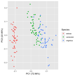
?ggfortify::autoplot.prcomplibrary(ggfortify) iris[1:2,] # Sepal.Length Sepal.Width Petal.Length Petal.Width Species # 1 5.1 3.5 1.4 0.2 setosa # 2 4.9 3.0 1.4 0.2 setosa df <- iris[1:4] # exclude "Species" column pca_res <- prcomp(df, scale. = TRUE) p <- autoplot(pca_res, data = iris, colour = 'Species') # OR turn off scaling on axes in order to get the same plot as the direct method # p <- autoplot(pca_res, data = iris, colour = 'Species', scale = 0) p # PC1 (72.96%), PC2 (22.85%) library(plotly) ggplotly(p)
Basic method
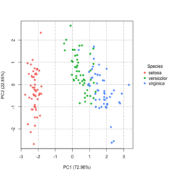
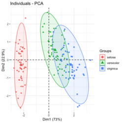
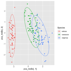
group <- as.numeric(iris$Species) # ggplot2's palette gg_color_hue <- function(n) { hues = seq(15, 375, length = n + 1) hcl(h = hues, l = 65, c = 100)[1:n] } n <- 3 # iris$Species has 3 levels cols = gg_color_hue(n) prp <- pca_res$sdev^2/ sum(pca_res$sdev^2) xlab <- paste0("PC1 (", round(prp[1]*100,2), "%)") ylab <- paste0("PC2 (", round(prp[2]*100,2), "%)") omar <- par(mar=c(5,4,4,8)) plot(pca_res$x[, 1], pca_res$x[, 2], xlab = xlab, ylab = ylab, col = cols[group], pch=16) grid(NULL, NULL, lty=3, lwd=1, col="#000000") par(xpd=TRUE) legend(4, 1, legend = levels(iris$Species), col=cols, pch=16, bty = "n", title = "Species") par(xpd=FALSE) par(omar)library(factoextra) fviz_pca_ind(pca_res, habillage=iris$Species, label = "none", ellipse.level=0.95, # default addEllipses=TRUE, title = "PCA") - Why the ellipses generated by fviz_pca_ind() and stat_ellipse() are different? How does R calculate the PCA ellipses?
- Compute normal data ellipses. Default is using the t-distribution.
- Plot PCA with ellipses using ggplot
- Error: Too few points to calculate an ellipse with 3 points? - R factoextra + ggforce packages
- Compute and draw an ellipse using base R functions. type ="norm" case.
# Example dataset data <- iris # ggplot2 method ggplot(data, aes(x = Sepal.Length, y = Sepal.Width)) + geom_point() + stat_ellipse(level = 0.95, type = "norm") + ggtitle("norm distribution") # Base R method # Select x and y variables x <- data$Sepal.Length y <- data$Sepal.Width # Calculate the mean of x and y mean_x <- mean(x) mean_y <- mean(y) # Create a covariance matrix cov_matrix <- cov(cbind(x, y)) # Calculate the eigenvalues and eigenvectors of the covariance matrix eigen_decomp <- eigen(cov_matrix) eig_val <- eigen_decomp$values eig_vec <- eigen_decomp$vectors # Set the confidence level confidence_level <- 0.95 # Get the number of observations n <- length(x) # Compute the scaling factor t_val <- sqrt(2 * qf(confidence_level, 2, n - 1)) # Generate points for the ellipse theta <- seq(0, 2 * pi, length.out = 100) ellipse_coords <- t(eig_vec %*% diag(sqrt(eig_val)) %*% rbind(cos(theta), sin(theta))) * t_val # Translate the ellipse to the mean ellipse_coords[,1] <- ellipse_coords[,1] + mean_x ellipse_coords[,2] <- ellipse_coords[,2] + mean_y # Plot the points and the ellipse plot(x, y, xlab = "Sepal Length", ylab = "Sepal Width", main = "Scatter Plot with Confidence Ellipse") lines(ellipse_coords, col = "red", lwd = 2) - Two categorical variables: one point shape and one fill color?
- PCA and Visualization
- Scree plots from the FactoMineR package (based on ggplot2)
- 2 lines of code, plotPCA() from DESeq2


Interactive Principal Component Analysis
- Use the identify() function and mouse clicks to label some points (also return the indices of these points).
- Interactive Principal Component Analysis in R
center and scale
What does it do if we choose center=FALSE in prcomp()?
In USArrests data, use center=FALSE gives a better scatter plot of the first 2 PCA components.
x1 = prcomp(USArrests)
x2 = prcomp(USArrests, center=F)
plot(x1$x[,1], x1$x[,2])  # looks random
windows(); plot(x2$x[,1], x2$x[,2]) # looks good in some sense
"scale. = TRUE" and Mean subtraction
- PCA is sensitive to the scaling of the variables. See PCA -> Further considerations.
- https://www.rdocumentation.org/packages/stats/versions/3.6.2/topics/prcomp
- By default scale. = FALSE in prcomp()
- By default, it centers the variable to have mean equals to zero. With parameter scale. = T, we normalize the variables to have standard deviation equals to 1. See also Normalizing all the variarbles vs. using scale=TRUE option in prcomp in R.
- Practical Guide to Principal Component Analysis (PCA) in R & Python
- What is the best way to scale parameters before running a Principal Component Analysis (PCA)?
- As a rule of thumb, if all your variables are measured on the same scale and have the same unit, it might be a good idea *not* to scale the variables (i.e., PCA based on the covariance matrix). If you want to maximize variation, it is fair to let variables with more variation contribute more. On the other hand, If you have different types of variables with different units, it is probably wise to scale the data first (i.e., PCA based on the correlation matrix).
- If all your variables are recorded in the same scale and/or the difference in variable magnitudes are of interest, you may choose not to normalize your data prior to PCA. See Normalizing all the variarbles vs. using scale=TRUE option in prcomp in R
- Let's compare the difference using the USArrests data
USArrests[1:3,]
#         Murder Assault UrbanPop Rape
# Alabama   13.2     236       58 21.2
# Alaska    10.0     263       48 44.5
# Arizona    8.1     294       80 31.0

pca1 <- prcomp(USArrests)  # inappropriate, default is scale. = FALSE
pca2 <- prcomp(USArrests, scale. = TRUE)
pca1$x[1:3, 1:3]
#               PC1        PC2       PC3
# Alabama  64.80216 -11.448007 -2.494933
# Alaska   92.82745 -17.982943 20.126575
# Arizona 124.06822   8.830403 -1.687448
pca2$x[1:3, 1:3]
#                PC1        PC2         PC3
# Alabama -0.9756604  1.1220012 -0.43980366
# Alaska  -1.9305379  1.0624269  2.01950027
# Arizona -1.7454429 -0.7384595  0.05423025

set.seed(1)
X <- matrix(rnorm(10*100), nr=10)
pca1 <- prcomp(X)
pca2 <- prcomp(X, scale. = TRUE)
range(abs(pca1$x - pca2$x))  # [1] 3.764350e-16 1.139182e+01
par(mfrow=c(1,2))
plot(pca1$x[,1], pca1$x[, 2], main='scale=F')
plot(pca2$x[,1], pca2$x[, 2], main='scale=T')
par(mfrow=c(1,1))
# rotation matrices are different
# sdev are different
# rotation matrices are different

# Same observations for a long matrix too
set.seed(1)
X <- matrix(rnorm(10*100), nr=100)
pca1 <- prcomp(X)
pca2 <- prcomp(X, scale. = TRUE)
range(abs(pca1$x - pca2$x))  # [1] 0.001915974 5.112158589

svd1 <- svd(USArrests)
svd2 <- svd(scale(USArrests, F, T))
svd1$d
# [1] 1419.06140  194.82585   45.66134   18.06956
svd2$d
# [1] 13.560545  2.736843  1.684743  1.335272
# u (or v) are also different
- Biplot
Number of components
Obtaining the number of components from cross validation of principal components regression
AIC/BIC in estimating the number of components
PCA and SVD
Using the SVD to perform PCA makes much better sense numerically than forming the covariance matrix to begin with, since the formation of [math]\displaystyle{ X X^T }[/math] can cause loss of precision.
- http://math.stackexchange.com/questions/3869/what-is-the-intuitive-relationship-between-svd-and-pca
- Relationship between SVD and PCA. How to use SVD to perform PCA?
R example
covMat <- matrix(c(4, 0, 0, 1), nr=2)
p <- 2
n <- 1000
set.seed(1)
x <- mvtnorm::rmvnorm(n, rep(0, p), covMat)
svdx <- svd(x)
result= prcomp(x, scale = TRUE)
summary(result)
# Importance of components:
#                          PC1    PC2
# Standard deviation     1.0004 0.9996
# Proportion of Variance 0.5004 0.4996
# Cumulative Proportion  0.5004 1.0000

# It seems scale = FALSE result can reflect the original data
result2 <- prcomp(x, scale = FALSE) # DEFAULT
summary(result2)
# Importance of components:
#                           PC1    PC2
# Standard deviation     2.1332 1.0065  ==> Close to the original data
                                     #  ==> How to compute
                              # sqrt(eigen(var(x))$values ) = 2.133203 1.006460
# Proportion of Variance 0.8179 0.1821  ==> How to verify
                                        # 2.1332^2/(2.1332^2+1.0065^2) = 0.8179
# Cumulative Proportion  0.8179 1.0000
result2$sdev
# 2.133203 1.006460    #  sqrt( SS(distance)/(n-1) )
result2$sdev^2 / sum(result2$sdev^2)
# 0.8179279 0.1820721
result2$rotation
#                PC1           PC2
# [1,]  0.9999998857 -0.0004780211
# [2,] -0.0004780211 -0.9999998857
result2$sdev^2 * (n-1)
# [1] 4546.004 1011.948   #  SS(distance)

# eigenvalue for PC1 = singular value^2
svd(scale(x, center=T, scale=F))$d
# [1] 67.42406 31.81113
svd(scale(x, center=T, scale=F))$d ^ 2  # SS(distance)
# [1] 4546.004 1011.948
svd(scale(x, center=T, scale=F))$d / sqrt(nrow(x) -1)
# [1] 2.133203 1.006460     ==> This is the same as prcomp()$sdev
svd(scale(x, center=F, scale=F))$d / sqrt(nrow(x) -1)
# [1] 2.135166 1.006617     ==> So it does not matter to center or scale
svd(var(x))$d
# [1] 4.550554 1.012961
svd(scale(x, center=T, scale=F))$v # same as result2$rotation
#               [,1]          [,2]
# [1,]  0.9999998857 -0.0004780211
# [2,] -0.0004780211 -0.9999998857
sqrt(eigen(var(x))$values )
# [1] 2.133203 1.006460
eigen(t(scale(x,T,F)) %*% scale(x,T,F))$values  # SS(distance)
# [1] 4546.004 1011.948
sqrt(eigen(t(scale(x,T,F)) %*% scale(x,T,F))$values ) # Same as svd(scale(x.T,F))$d
# [1] 67.42406 31.81113.

# So SS(distance) = eigen(t(scale(x,T,F)) %*% scale(x,T,F))$values
#                 = svd(scale(x.T,F))$d ^ 2
Related to Factor Analysis
- http://www.aaronschlegel.com/factor-analysis-introduction-principal-component-method-r/.
- http://support.minitab.com/en-us/minitab/17/topic-library/modeling-statistics/multivariate/principal-components-and-factor-analysis/differences-between-pca-and-factor-analysis/
In short,
- In Principal Components Analysis, the components are calculated as linear combinations of the original variables. In Factor Analysis, the original variables are defined as linear combinations of the factors.
- In Principal Components Analysis, the goal is to explain as much of the total variance in the variables as possible. The goal in Factor Analysis is to explain the covariances or correlations between the variables.
- Use Principal Components Analysis to reduce the data into a smaller number of components. Use Factor Analysis to understand what constructs underlie the data.
prcomp vs princomp
prcomp vs princomp from sthda. prcomp() is preferred compared to princomp().
Missing data
pcaMethods package from Bioconductor
ibrary(pcaMethods)

X <- as.matrix(iris[, 1:4])   # complete numeric data (no NAs)

## 2) PCA with pcaMethods (BPCA, 2 PCs)
# "uv" → unit variance scaling
set.seed(1)
res_bpca <- pca(X, method = "bpca", nPcs = 2, center = TRUE, scale = "uv")

scores_bpca <- scores(res_bpca)
ve_bpca     <- res_bpca@R2 * 100   # % variance explained

## 3) Regular PCA with prcomp (2 PCs)
pr <- prcomp(X, center = TRUE, scale. = TRUE)

scores_pr <- pr$x[, 1:2]
ve_pr     <- (pr$sdev^2 / sum(pr$sdev^2)) * 100

ve_bpca # [1] 72.89531 22.63549
ve_pr   # [1] 72.9624454 22.8507618  3.6689219  0.5178709

## 4) Plot comparison
op <- par(mfrow = c(1, 2))

plot(scores_bpca[,1], scores_bpca[,2],
     xlab = sprintf("BPCA PC1 (%.1f%%)", ve_bpca[1]),
     ylab = sprintf("BPCA PC2 (%.1f%%)", ve_bpca[2]),
     pch = 19, main = "pcaMethods: bpca (2 PCs)")

plot(scores_pr[,1], scores_pr[,2],
     xlab = sprintf("prcomp PC1 (%.1f%%)", ve_pr[1]),
     ylab = sprintf("prcomp PC2 (%.1f%%)", ve_pr[2]),
     pch = 19, main = "prcomp (2 PCs)")

par(op)
Relation to Multidimensional scaling/MDS
With no missing data, classical MDS (Euclidean distance metric) is the same as PCA.
Comparisons are here.
Differences are asked/answered on stackexchange.com. The post also answered the question when these two are the same.
isoMDS (Non-metric)
cmdscale (Metric)
Matrix factorization methods
http://joelcadwell.blogspot.com/2015/08/matrix-factorization-comes-in-many.html Review of principal component analysis (PCA), K-means clustering, nonnegative matrix factorization (NMF) and archetypal analysis (AA).
Outlier samples
Detecting outlier samples in PCA
Reconstructing images
Reconstructing images using PCA
Sparse PCA
- https://en.wikipedia.org/wiki/Sparse_PCA
- 8.6.1 Sparse Principal Components from Harrell's "Regression Modeling Strategies" book
- pcaPP package
Misc
PCA for Categorical Variables
- FAMD - Factor Analysis of Mixed Data in R: Essentials
- PCA for Categorical Variables in R. Factorial Analysis of Mixed Data (FAMD) Is a PCA for Categorical Variables Alternate.
psych package
Principal component analysis (PCA) in R
glmpca: Generalized PCA for dimension reduction of sparse counts
Feature selection and dimension reduction for single-cell RNA-Seq based on a multinomial model