GSEA
Basic
https://en.wikipedia.org/wiki/Gene_set_enrichment_analysis
Determines whether an a priori defined set of genes shows statistically significant, concordant differences between two biological states
- https://www.bioconductor.org/help/course-materials/2015/SeattleApr2015/E_GeneSetEnrichment.html, https://www.bioconductor.org/help/course-materials/2009/SeattleApr09/gsea/HyperG_Lecture.pdf. For hypergeometric test, it is
- finding Biocarta or KEGG pathways significantly enriched in the user's gene list
- Are DE genes in the set more common than DE genes not in the set?.
- Are selected genes more often in the GO category than expected by chance? (one-tailed)
We can draw a 2x2 table or a venn diagram to see the diagram.
In gene set Yes No DE Yes No
- Gene List Enrichment Analysis dhyper(), binom.test(), fisher.test().
- Enrichment or depletion of a GO category within a class of genes: which test? Rivals 2007
- Pathway Commons
- A positive enrichment score indicates that the gene set is overrepresented at the top of the ranked list. This means that the genes in the set are more likely to be up-regulated, with relatively small p-values.
- A negative enrichment score suggests that the gene set is overrepresented at the bottom of the ranked list. This implies that the genes in the set are more likely to be down-regulated.
- Gene set analysis methods: statistical models and methodological differences 2014
- http://software.broadinstitute.org/gsea/index.jsp, Subramanian, et al 2005 paper
- HOW TO PERFORM GSEA - A tutorial on gene set enrichment analysis for RNA-seq (video)
- Algorithm. GSEA walks down the ranked list of genes, increasing a running-sum statistic when a gene belongs to the set and decreasing it when the gene does not.
- Interpretation of 3 enrichment plots. The 1st plot (ES on y-axis) tells you how over or under expressed is your gene respect to the ranked list. The 2nd part of the graph (barcode-like) shows where the members of the gene set appear in the ranked list of genes. The 3rd graph (y=ranked list metric, x=rank) shows how your metric is distributed along the list.
- slides with formulas.
- What does a negative enrichment score mean? A negative NES will indicate that the genes in the set S will be mostly at the bottom of your list L.
- GSEA R Implementation from GSEA-MSigDB.
- READMe.
- Using GSEA.1.0.R
- Statistical power of gene-set enrichment analysis is a function of gene set correlation structure by SWANSON 2017
- clusterProfiler package and the online book.
- Gene-set Enrichment with Regularized Regression Fang 2019
- msigdbr package. MSigDB Gene Sets for Multiple Organisms in a Tidy Data Format.
- Best method/package for Gene Set Enrichment Analysis in R? and the gage package
- ES could be negative; see Genome 559: Introduction to Statistical and Computational Genomics
- multiGSEA: a GSEA-based pathway enrichment analysis for multi-omics data
- How to use DAVID for functional annotation of genes, Using DAVID for Functional Enrichment Analysis in a Set of Genes (Part 1), (Part 2) (video)
Two categories of GSEA procedures:
- Competitive: compare genes in the test set relative to all other genes.
- Self-contained: whether the gene-set is more DE than one were to expect under the null of no association between two phenotype conditions (without reference to other genes in the genome). For example the method by Jiang & Gentleman Bioinformatics 2007
See also BRB-ArrayTools -> GSEA.
Hypergeometric test
- Suppose you have a bag with 100 balls, 20 of which are red and the rest are blue. You draw 10 balls from the bag without replacement. Let’s say 4 of these balls are red. You want to know if drawing 4 red balls out of 10 is significantly different from random chance.
Here’s how you would set up the hypergeometric test:- Define the Universe (N): The total number of balls, which is 100.
- Define the Gene Set (M): The total number of red balls, which is 20.
- Define the Number of Successes (DE genes) in the Universe (n): The number of balls you drew, which is 10.
- Define the Number of Successes (DE genes) in the Gene Set (x): The number of red balls you drew, which is 4.
N=100 +-----------------------------+ | M=20 n=10 | | (# in a pathway) (# of DE) | | +-------+--------+-------+ | | | | x=4 | | | | | | common | | | | +-------+--------+-------+ | +-----------------------------+ OR N=100 ------> Draw n=10 +--------+ +--------+ | | | | | | | | x=4 | | M=20 +--------+ (in a pathway) +--------+ (some pathway) OR +----------------------+ | C(20, 4) * C(80, 6) | +----------------------+ Probability = ---------------------------- +----------------------+ | C(100, 10) | +----------------------+ - R code illustration ?phyper:
dhyper(x, m, n, k, log = FALSE)
# p(x) = C(m, x) C(n, k-x) / C(m+n, k)

# m: the number of white balls in the urn.
# n: the number of black balls in the urn.
# k: the number of balls drawn from the urn.
# x: the number of white balls drawn without replacement
N <- 1000
M <- 200
n <- 50
x <- 20

# Probability of observing 20 or more DEGs in the pathway by chance,
#            given the background gene set and the pathway gene set.
p <- 0; for(i in 20:50) p <- p + dhyper(i, M, N - M, n) # P(X >= 20)
# 0.0006763799

phyper(19, M, N - M, n, lower.tail = FALSE) # P(X > 19), not P(X >= 19)
# 0.0006763799

1 - phyper(19, M, N - M, n, lower.tail = T) # 1 - P(X <= 19), default is lower.tail=T
# 0.0006763799
- In the context of gene set enrichment analysis,
- Define the Universe (N): The total number of genes that you have profiled in your experiment. Let’s say you have profiled 20,000 genes.
- Define the Gene Set (M): The total number of genes known to be involved in a specific biological pathway. For example, suppose there are 200 genes known to be involved in the “cell cycle” pathway.
- Define the Number of Successes (DE genes) in the Universe (n): The number of genes that are differentially expressed in your experiment. Let’s say you found 2,000 genes to be differentially expressed.
- Define the Number of Successes (DE genes) in the Gene Set (x): The number of differentially expressed genes that are also in your gene set. Suppose 50 of the 2,000 differentially expressed genes are involved in the “cell cycle” pathway.
    N=20,000
   +-----------------------------+
   |   M=200             n=2000  |
   | (# in a pathway)  (# of DE) |
   |  +-------+--------+-------+ |
   |  |       |  x=50  |       | |
   |  |       | common |       | |
   |  +-------+--------+-------+ |
   +-----------------------------+
We calculate the tail probability to report the p-value; [math]\displaystyle{ P(X \geq 50) = P(X=50) + \cdots + P(X=min(M, n)) }[/math]. If this p-value is below a certain threshold (commonly 0.05), we reject the null hypothesis and conclude that the pathway is significantly enriched among the differentially expressed genes. It’s also important to remember that statistical significance does not always imply biological significance, and further validation is often required.</math>
Interpretation
- Gene Set Enrichment Analysis (GSEA) takes an alternative approach : it focuses on cumulative changes in expression of multiple genes as a group (belonging to a same gene-set/pahtway), which shifts the focus from individual genes to groups of genes. See this.
- XXX class/subtype is associated with the OOO gene set(s) (GSVA vignette)
- XXX subtype (of samples) is characterized by the expression of OOO markers, thus we expect it to correlate with the OOO2 gene set (GSVA vignette)
- The XXX subtype (of samples) shows high expression of OOO genes, thus the OOO gene set is highly enriched for this group (GSVA vignette). OR if we find a gene set is enriched in XXX subtype (e.g. sensitive models), it means genes in that gene set are more highly expressed in the XXX subtype samples compared to the YYY subtype samples.
- Negative ES Interpretation.
- A positive enrichment score should always reflect enrichment on the positive side of the zero cross (although not necessarily all genes on the positive side) and be enrichment in whichever phenotype was selected to be first in the comparison in the Phenotype selection dialogue. And vice versa, with a negative enrichment score reflecting enrichment in the genes on the negative side of the ranked list.
- GSEA is known to have some issues with highly skewed gene distributions, but that shouldn't affect the raw enrichment scores, just NES and significance calculations when GSEA runs in to a condition where its only sampled from one side of the distribution.
- Enrichment Score Interpretation
- If, for example, you provide a gene list ranked by a combination of fold change and p-value (e.g., sign(FC) * log10(pvalue)), then the positive scores are associated with upregulated genes and negative scores are associated with downregulated genes.
- fgsea paper
- The more positive is the value of sr(p) the more enriched the gene set is in the positively-regulated genes (with Si > 0). Accordingly, negative sr(p) corresponds to enrichment in the negatively regulated genes.
- The opposite of "enriched" is "depleted". See Wikipedia.
Calculation
- Subramanian paper
- https://youtu.be/bT00oJh2x_4
- *pathwaycommons.org
- Compute cumulative sum over ranked genes. MD Anderson lecture
- Increase sum when gene in set, decrease it otherwise. That is, +1/-1 weights in cumulative sum is used to represent whether genes are in the interested gene set.
- Magnitude of increment depends on correlation of gene with phenotype.
- Record the maximum deviation from zero as the enrichment score
FDR cutoff
Why does GSEA use a false discovery rate (FDR) of 0.25 rather than the more classic 0.05?
Given the lack of coherence in most expression datasets and the relatively small number of gene sets being analyzed, using a more stringent FDR cutoff may lead you to overlook potentially significant results.
GSEAtraining
https://jokergoo.github.io/GSEAtraining/
piano
- piano package. Platform for integrative analysis of omics data.
- Available GSA methods.
- The main function is runGSA(). It contains a wide range of GSEA methods like maxmean, fisher, gsea, fgsea, etc.
- Conceptual overview of the runGSA workflow
- It was used in Xeva paper.
edgeR
Over-representation analysis. ?goana and ?kegga. See UserGuide 2.14 Gene ontology (GO) and pathway analysis.
fgsea
fgsea package and download stat
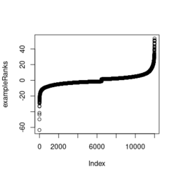
- ?exampleRanks gives a hint about how it was obtained. It is actually the t-statistic, not logFC.
... fit2 <- eBayes(fit2) de <- data.table(topTable(fit2, adjust.method="BH", number=12000, sort.by = "B"), keep.rownames = TRUE) colnames(de) plot(de$t, exampleRanks[match(de$rn, names(exampleRanks))]) # 45 degrees straight line range(de$t) # [1] -62.22877 52.59930 range(exampleRanks) # [1] -63.33703 53.28400 range(de$logFC) # [1] -11.56067 12.57562 - Paper is still on biorxiv only. Scholar.google.com. Computer tech lab in Russia.
- Documentation
- ?collapsePathways. Collapse list of enriched pathways to independent ones.
- DESeq results to pathways in 60 Seconds with the fgsea package
- Performing GSEA using MSigDB gene sets in R
- Using the fast preranked gene set enrichment analysis (fgsea) package
Are fgsea and Broad Institute GSEA equivalent
Are fgsea and Broad Institute GSEA equivalent?
Examples
- vignette,
- plotEnrichment() for a single pathway (including the output plot). No need to run fgsea(). Source code. Enrichment score (ES) on the plot is calculated by calcGseaStat()$res. The ES value is the same as the one shown in plotGseaTable() though plotEnrichment does not return it.
- plotGseaTable() for a bunch of selected pathways (including the output plot).
- Basic usage
library(fgsea)
library(ggplot2)
data(examplePathways) # a list of length 1457 (pathways)
data(exampleRanks)    # a vector of length 12000 (genes)
set.seed(42)
fgseaRes <- fgsea(pathways = examplePathways,
                   stats    = exampleRanks,
                   minSize  = 4, # default minSize=1, maxSize=Inf
                   maxSize  =10)
# I used a very small maxSize in order to see details later
# So the results here can't be compared with the default
class(fgseaRes)
# [1] "data.table" "data.frame"
dim(fgseaRes)
# [1] 386   8
fgseaRes[1:2, ]
#                                                          pathway      pval      padj
# 1:                        1368092_Rora_activates_gene_expression 0.8630705 0.9386018
# 2: 1368110_Bmal1:Clock,Npas2_activates_circadian_gene_expression 0.4312268 0.8159487
#       log2err         ES        NES size              leadingEdge
# 1: 0.05412006 -0.3087414 -0.6545067    5 11865,12753,328572,20787
# 2: 0.08312913  0.4209054  1.0360288    9        20893,59027,19883

sapply(examplePathways, length) |> range()
# [1]    1 2366
# Question: minSize, maxSize mean 'matched' genes? Can't verify
sum(sapply(examplePathways, length) < 3)
# [1] 104
sum(sapply(examplePathways, length) > 10)
# [1] 939
1457 - 104 - 939
# [1] 414
examplePathways2 <- lapply(examplePathways, function(x) x[x %in% names(exampleRanks)])
sapply(examplePathways2, length) |> range()
# [1]   0 968
sum(sapply(examplePathways2, length) < 3)
# [1] 232
sum(sapply(examplePathways2, length) > 10)
# [1] 730
1457 - 232 - 730
# [1] 495
range(fgseaRes$ES)
# [1] -0.8442416  0.9488163
range(fgseaRes$NES)
# [1] -2.020695  2.075729
order(fgseaRes$ES)[1:5]
# [1]  75 289 320 249 312
order(fgseaRes$NES)[1:5]
# [1] 289  75 102 320 200

# choose the top gene set in order to zoom in & see the detail
head(fgseaRes[order(pval), ], 1)
#                            pathway         pval         padj   log2err        ES
# 1: 5991601_Phosphorylation_of_Emi1 2.461461e-07 9.501241e-05 0.6749629 0.9472236
#         NES size                           leadingEdge
# 1: 2.082967    6 107995,12534,18817,67141,268697,56371

plotEnrichment(examplePathways[["5991601_Phosphorylation_of_Emi1"]], exampleRanks)
# 12000 total genes though only 6 genes are matched in this top gene set.
debug(plotEnrichment)
# Browse[2]> toPlot
#        x            y
# 1      0  0.000000000
# 2     47 -0.003918626
# 3     48  0.308356695
# 4    322  0.285511939
# 5    323  0.452415897
# 6    407  0.445412396
# 7    408  0.593677191
# 8    447  0.590425565
# 9    448  0.730277162
# 10   617  0.716186784
# 11   618  0.833696389
# 12   638  0.832028888
# 13   639  0.947223612
# 14 12001  0.000000000
examplePathways[["5991601_Phosphorylation_of_Emi1"]]
# [1] "12534"     "18817"     "56371"     "67141"     "107995"    "268697"
# [7] "434175"    "102643276"
match(examplePathways[["5991601_Phosphorylation_of_Emi1"]], names(exampleRanks))
# [1] 11678 11593 11362 11553 11953 11383    NA    NA
# Since there are 12000 total genes and exampleRanks have been sorted,
# these matched genes have very high ranks.
# See the plot below.

length(exampleRanks)
# [1] 12000
exampleRanks[1:10]
#    170942    109711     18124     12775     72148     16010     11931
# -63.33703 -49.74779 -43.63878 -41.51889 -33.26039 -32.77626 -29.42328
#     13849    241230    665113
# -28.83475 -28.65111 -27.81583
sum(exampleRanks < 0)
# [1] 6469
sum(exampleRanks > 0)
# [1] 5531
plot(exampleRanks)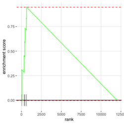
There are 6*2 points (excluding the 0 value at the starting and end) in the figure.
- The range of NES is not [-1, 1] but ES seems to be in [-1, 1]. The example sort pathways by NES but it can be adapted to sort by pval. Source code. Also ES and NES are not in the same order (see below) though we cannot tell it from the small plot. According to the manual,
- ES – enrichment score, same as in Broad GSEA implementation;
- NES – enrichment score normalized to mean enrichment of random samples of the same size (the number of genes in the gene set).
- Hπow to interpret NES(normalized enrichment score)?
- Negative normalized Enrichment Score (NES) in GSEA analysis
- question about GSEA about the sign of ES/NES. "Does this means in positive NES upregulated genes are enriched while in negative NES DN genes are enriched?"π Step 1. rank all genes in your list (L) based on "how well they divide the conditions". Step 2, you want to see whether the genes present in a gene set (S) are at the top or at the bottom of your list...or if they are just spread around randomly. A positive NES will indicate that genes in set S will be mostly represented at the top of your list L. a negative NES will indicate that the genes in the set S will be mostly at the bottom of your list L.
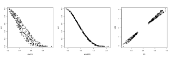
with(fgseaRes, plot(abs(ES), pval))  # relationship is not consistent for a lot of pathways
with(fgseaRes, plot(abs(NES), pval)) # relationship is more consistent
with(fgseaRes, plot(ES, NES))

head(order(fgseaRes$pval))
# [1] 121 112 289  68 187 188
head(rev(order(abs(fgseaRes$NES))))
# [1] 121 289  68 188 187  22
- The computation speed is FAST!
system.time(invisible(fgsea(examplePathways, exampleRanks)))
#    user  system elapsed
#  31.162  38.427  15.800


plotEnrichment()
- Understand plotEnrichment() function. Plot shape (concave or convex) requires the stats of genes from both in- and out- of the gene set. This affects the interpretation of the plot. The plot always starts with 0 and end with 0 in Y (enrichment score). plotEnrichment() does not return enrichment scores even it calculates them for the plot.
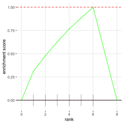
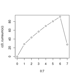
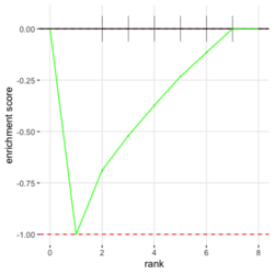
# Reduce the total number of genes
i <- match(examplePathways[["5991601_Phosphorylation_of_Emi1"]], names(exampleRanks))
i <- na.omit(i)   # Exclude 2 genes in the pathways but not in the data

if (FALSE) {
  # Total genes = pathway genes will not work?
  plotEnrichment(examplePathways[["5991601_Phosphorylation_of_Emi1"]], exampleRanks[i])
  # Error: GSEA statistic is not defined when all genes are selected
}

# PS values in 'exampleRanks' object are sorted from the smallest to the largest

# Case 1: include 1 down-regulated gene for our total genes
plotEnrichment(examplePathways[["5991601_Phosphorylation_of_Emi1"]], exampleRanks[c(1,i)])
# saved as fgseaPlotSmall.png
exampleRanks[c(1,i)]
#    170942     12534     18817     56371     67141    107995    268697
# -63.33703  15.16265  13.46935  10.46504  12.70504  28.36914  10.67534
#
# Rank and add +1/-1,
# 28.36 15.16 13.46 12.70 10.67 10.46 -63.33
#    +1    +1    +1    +1    +1    +1     -1
debug(plotEnrichment)
# Browse[2]> toPlot
#    x         y
# 1  0 0.0000000
# 2  0 0.0000000
# 3  1 0.3122753
# 4  1 0.3122753
# 5  2 0.4791793
# 6  2 0.4791793
# 7  3 0.6274441
# 8  3 0.6274441
# 9  4 0.7672957
# 10 4 0.7672957
# 11 5 0.8848053
# 12 5 0.8848053
# 13 6 1.0000000
# 14 8 0.0000000
x <-c(28.36, 15.16, 13.46, 12.70, 10.67, 10.46, -63.33)
plot(0:7, c(0, cumsum(x)), type = "b")

# Case 2: include another one up-regulated gene (so all are up-reg) for our total genes
# However, the largest gene (added) is not in the gene set.
# It will make the plot starting from a negative value (ignore 0 from the very left)
plotEnrichment(examplePathways[["5991601_Phosphorylation_of_Emi1"]], exampleRanks[c(i, 12000)])
# saved as fgseaPlotSmall2.png
exampleRanks[c(i, 12000)]
#    12534    18817    56371    67141   107995   268697    80876
# 15.16265 13.46935 10.46504 12.70504 28.36914 10.67534 53.28400
#
# Rank and add +1/-1
# 53.28 28.36  15.16 13.46 12.70 10.67 10.46
#    -1    +1     +1    +1    +1    +1    +1
For figure 1 (case 1), it has 6 points. Figure 2 is the one I generate using plot() and exampleRanks. For figure 3 (case 2), it has 7 points (excluding the 0 value at the starting and end). The curve goes down first because the gene has the largest rank (statistic) and is not in the pathway. So the x-axis location is determined by the rank/statistics and going up or down on the y-axis is determined by whether the gene is in the pathway or not.
 ,
,  ,
, 
- Shifting exampleRanks values will change the enrichment scores because the directions of genes' statistics change?
plotEnrichment(examplePathways[[1]],
                exampleRanks) + labs(title="Programmed Cell Death")
            # like sin() with one period
range(exampleRanks)
# [1] -63.33703  53.28400
plotEnrichment(examplePathways[[1]],
                exampleRanks+64) + labs(title="Programmed Cell Death")
            # like a time series plot
plotEnrichment(examplePathways[[1]],
                exampleRanks-54) + labs(title="Programmed Cell Death")
            # same problem if we shift exampleRanks to all negative
including NE, NES, pval, etc. So it is not purely rank-based.
set.seed(42)
fgseaRes2 <- fgsea(pathways = examplePathways,
                   stats    = exampleRanks+2, # OR 2*(exampleRanks+2)
                   minSize  = 4,
                   maxSize  =10)
identical(fgseaRes, fgseaRes2)
# [1] FALSE
R> fgseaRes[1:3, c("ES", "NES", "pval")]
           ES        NES      pval
1: -0.3087414 -0.6545067 0.8630705
2:  0.4209054  1.0360288 0.4312268
3: -0.4065043 -0.8617561 0.6431535
R> fgseaRes2[1:3, c("ES", "NES", "pval")]
           ES        NES      pval
1:  0.4554877  0.8284722 0.7201767
2:  0.5520914  1.1604366 0.2833333
3: -0.2908641 -0.5971951 0.9442724
However, scaling won't change anything (because scaling does not change the directions?).
set.seed(42)
fgseaRes3 <- fgsea(pathways = examplePathways,
                   stats    = 2*exampleRanks,
                   minSize  = 4,
                   maxSize  =10)
identical(fgseaRes, fgseaRes3)
# [1] TRUE


plotGseaTable()
- Obtain enrichment scores by calling fgsea(); i.e. fgseaMultilevel().
examplePathways[["5991601_Phosphorylation_of_Emi1"]] |> length() # [1] 8 set.seed(1) fgsea2 <- fgsea(pathways = examplePathways["5991601_Phosphorylation_of_Emi1"], stats = exampleRanks) tibble::as_tibble(fgsea2) # A tibble: 1 × 8 # pathway pval padj log2err ES NES size leadi…¹ # <chr> <dbl> <dbl> <dbl> <dbl> <dbl> <int> <list> # 1 5991601_Phosphor… 9.39e-7 9.39e-7 0.659 0.947 2.05 6 <chr> # … with abbreviated variable name ¹leadingEdge plotGseaTable(examplePathways["5991601_Phosphorylation_of_Emi1"], exampleRanks, fgsea2)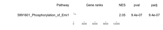
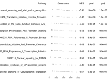
The signs of NES/ES can be confirmed from the gene rank plot. Below is a plot from 10 enriched pathways
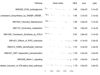
and a plot from 10 non-enriched pathways


Subramanian algorithm
In the plot, (x-axis) genes are sorted by their expression across all samples. Y-axis represents enrichment score. See HOW TO PERFORM GSEA - A tutorial on gene set enrichment analysis for RNA-seq. Bars represents genes being in the gene set. Genes on the LHS/RHS are more highly expressed in the experimental/control group. Small p means this gene set is enriched in this experimental sample.
Kolmogorov Smirnov test statistic
- In Gene Set Enrichment Analysis (GSEA), the Kolmogorov-Smirnov test is used to calculate an enrichment score for each gene-set (pathway).
- This score reflects how often members (genes) included in that gene-set (pathway) occur at the top or bottom of the ranked data set.
- The ranking is based on a measure of differential gene expression.
- The enrichment score is calculated using the Kolmogorov-Smirnov statistic, which quantifies the distance between the empirical distribution function of a sample and the cumulative distribution function of a reference distribution, or between the empirical distribution functions of two samples.
- In GSEA, the empirical distribution function represents the ranked list of genes, and the reference distribution represents the gene-set (pathway) being tested for enrichment.
- The enrichment score is then used to determine whether the gene-set (pathway) is significantly enriched in the ranked list of genes.
- An example
- Let’s say we have a ranked list of 10 genes based on their differential expression between two conditions, with the most highly expressed genes at the top and the least expressed genes at the bottom. The list might look like this: GeneA, GeneB, GeneC, GeneD, GeneE, GeneF, GeneG, GeneH, GeneI, GeneJ.
- Now let’s say we have a gene-set (pathway) that contains three genes: GeneB, GeneD, and GeneH. We want to determine if this gene-set is significantly enriched in our ranked list of genes.
- To do this, we can use the Kolmogorov-Smirnov test to calculate an enrichment score for the gene-set. The test will calculate the maximum distance between the empirical distribution function of our ranked list of genes and the cumulative distribution function of our gene-set.
- The empirical distribution function of our ranked list of genes is a step function that increases by 1/10 at each gene in the list. The cumulative distribution function of our gene-set is also a step function that increases by 1/3 at each gene in the set.
- The Kolmogorov-Smirnov statistic will then calculate the maximum vertical distance between these two functions. If this distance is large, it suggests that the members of our gene-set (GeneB, GeneD, and GeneH) are occurring more often at the top or bottom of our ranked list of genes than would be expected by chance. This would indicate that our gene-set is significantly enriched in our ranked list of genes.
- To determine if the distance is statistically significant, we can compare the calculated KS statistic to a critical value obtained from a reference distribution. If the KS statistic is greater than the critical value, we can conclude that the gene-set is significantly enriched in the ranked list of genes.
- What is the reference distribution of KS statistic? In the context of Gene Set Enrichment Analysis (GSEA), the reference distribution for the Kolmogorov-Smirnov (KS) statistic is obtained by permuting the sample labels (resampling genes actually) and recalculating the enrichment score for the gene-set many times. This creates a null distribution of enrichment scores that represents what we would expect to see if the gene-set was not enriched in the ranked list of genes.
- The critical value for the KS statistic is then obtained from this null distribution, typically by taking a high percentile (e.g., the 95th percentile) of the distribution. If the observed KS statistic is greater than this critical value, we can conclude that the gene-set is significantly enriched in the ranked list of genes.
- Why do we need to rank genes first? The ranking of genes is also used in the calculation of the enrichment score for a gene-set. The enrichment score reflects how often members (genes) included in that gene-set (pathway) occur at the top or bottom of the ranked list of genes. If the members of a gene-set occur more often at the top or bottom of the ranked list of genes than would be expected by chance, it suggests that the gene-set is significantly enriched in the ranked list of genes.
- R
# Define a ranked list of genes based on their differential expression
# between two conditions, with the most highly expressed genes at the top
# and the least expressed genes at the bottom
ranked_genes <- c("GeneA", "GeneB", "GeneC", "GeneD", "GeneE",
                  "GeneF", "GeneG", "GeneH", "GeneI", "GeneJ")

# Define a gene-set (pathway) that contains three genes
gene_set <- c("GeneB", "GeneD", "GeneH")

# Calculate the enrichment score for the gene-set using the KS statistic
enrichment_score <- max(ks.test(ranked_genes, gene_set)$statistic)

# Permute the sample labels and recalculate the enrichment score many times
# to create a null distribution of enrichment scores
set.seed(123)
n_permutations <- 1000
null_distribution <- replicate(n_permutations, {
  permuted_genes <- sample(ranked_genes)
  ks.test(permuted_genes, gene_set)$statistic
})

# Calculate the critical value for the KS statistic from the null distribution
critical_value <- quantile(null_distribution, 0.95)

# Determine if the gene-set is significantly enriched in the ranked list of genes
if (enrichment_score > critical_value) {
  print("The gene-set is significantly enriched in the ranked list of genes.")
} else {
  print("The gene-set is not significantly enriched in the ranked list of genes.")
}
pathlinkR
Facilitating pathway and network based analysis of RNA-Seq data with pathlinkR. It provides an integrated approach to performing pathway enrichment and network-based analyses, while also producing publication-quality figures to summarize these results, allowing users to more efficiently interpret their findings and extract biological meaning from large amounts of data. Bioconductor.
mulea
Rafael A Irizarry
Gene set enrichment analysis made simple
microRNA/miRNA
- https://en.wikipedia.org/wiki/MicroRNA 小分子核糖核酸
- miRNAmeConverter - Convert miRNA Names to Different miRBase Versions
- MicroRNAs (miRNAs) are a class of small, non-coding RNA molecules (無法進一步轉譯成蛋白質的RNA) that play a role in the regulation of gene expression. They are typically 21-23 nucleotides in length and are found in plants, animals, and some viruses. miRNAs function by binding to complementary sequences in messenger RNA (mRNA) molecules, leading to the silencing of the target gene through the degradation of the mRNA or the inhibition of its translation into protein.
- The expression of microRNAs (miRNAs) and their target mRNAs are often inversely correlated.
- This interaction results in the reduction of mRNA and/or protein levels.
- Therefore, when a miRNA is highly expressed, the level of its target mRNA is usually low, and vice versa. See Joint analysis of miRNA and mRNA expression data, miRNA Regulated Gene Expression in SARS-CoV-2 Research.
- MicroRNAs (miRNAs) are small non-coding RNAs that play a crucial role in regulating gene expression. They typically do this by binding to messenger RNAs (mRNAs) and preventing them from being translated into proteins. If a pathway undergoes less miRNA inhibition, it means that the miRNAs are not binding to the mRNAs as much, which could allow more protein to be produced.
- It is also important to note that one miRNA can target multiple mRNAs, and one mRNA can be targeted by multiple miRNAs.
- In the context of miRNAs, the term “target” refers to the specific mRNA molecules that a miRNA interacts with. When a miRNA binds to its target mRNA, it can inhibit the translation of the mRNA into protein or lead to the degradation of the mRNA. This is why the expression levels of a miRNA and its target mRNA are often inversely correlated. So, when I mentioned “target” in the last sentence, I was referring to the mRNA molecules that are regulated by the miRNA.
- A target gene is a gene whose expression is regulated by a specific regulatory molecule, such as a transcription factor or a microRNA. The regulatory molecule binds to specific sequences in the DNA or RNA of the target gene, leading to changes in the expression of that gene. For example, a transcription factor may bind to the promoter region of a target gene, leading to an increase or decrease in the transcription of that gene into messenger RNA (mRNA). Similarly, a microRNA may bind to the mRNA of a target gene, leading to the degradation of the mRNA or the inhibition of its translation into protein.
- MiRNAs are involved in a wide range of cellular processes, including cell growth, differentiation, development, and apoptosis, and have been implicated in many diseases
- miRScore: A rapid and precise microRNA validation tool 2025
RBiomirGS
- RBiomirGS R package which is based on logistic regressions with binary predictor variable (two groups).
Tip: The original instruction "devtools::install_github("jzhangc/git_RBiomiRGS/RBiomirGS", repos = BiocInstaller::biocinstallRepos())" is outdated because BiocInstaller has been replaced by the BiocManager package. The instruction on Github is correct.
Note: installing RBiomirGS on R 4.3.3 (BiocManager::version() = "3.18" and R 4.5.1 (BiocManager::version() = "3.21") on Windows works. There is no need to install Rtools.# R 4.3.3 docker run -it --rm --user rstudio bioconductor/bioconductor_docker:RELEASE_3_18 R devtools::install_github("jzhangc/git_RBiomiRGS/RBiomirGS", ref = "74a567a", repos = BiocManager::repositories()) # version 0.2.19, as of 4/17/2024 - Model:
- miRNA score: The score for each miRNA is calculated by combining significance and direction of change:
[math]\displaystyle{ S_{\text{mirna}} = -\log_{10}(p)\times \operatorname{sign}(\log_2\text{FC}) }[/math] where [math]\displaystyle{ p }[/math] is the p-value for the miRNA and [math]\displaystyle{ FC }[/math] is fold change. - mRNA score: The mRNA score aggregates contributions from interacting miRNAs:
[math]\displaystyle{ S_{\text{mrna}} = -\sum_{i=1}^{n} w(i)\times S_{\text{mirna},i} }[/math] [math]\displaystyle{ n }[/math] is the number of miRNAs predicted to interact with the mRNA. [math]\displaystyle{ w(i) }[/math] is an optional interaction weight (default = 1). The leading negative sign represents the inhibitory effect of miRNAs on mRNA. - The logistic model tests whether gene-set membership can be predicted from the mRNA score.
[math]\displaystyle{ P(Y=1\mid S_{\text{mrna}})=\frac{1}{1+\exp\big(-(\theta_0+\theta_1 S_{\text{mrna}})\big)} }[/math]
Equivalently (log-odds form): [math]\displaystyle{ \log\frac{P(Y=1)}{1-P(Y=1)}=\theta_0+\theta_1 S_{\text{mrna}} }[/math]. [math]\displaystyle{ Y=1 }[/math] indicates membership in the gene set. [math]\displaystyle{ \theta_1 }[/math] is the coefficient of interest: a positive value means higher [math]\displaystyle{ S_{mrna} }[/math] is associated with increased odds of membership. - If we have n gene sets, we will fit n logistic regressions.
- For each gene sets, we will use a logistic regression using data {[math]\displaystyle{ {(X_i, Y_i), i=1, ..., g} }[/math]}, where [math]\displaystyle{ X_i=S_{\text{mrna},i} }[/math] and [math]\displaystyle{ Y_i=1 }[/math] if gene [math]\displaystyle{ i }[/math] is in the gene set.
- RBiomirGS starts from miRNA differential expression, then maps those miRNAs to their predicted or validated target mRNAs.
- Hypothesis: Do genes with higher (or lower) mRNA scores tend to belong to this gene set more often than expected? OR
What pathways are likely being activated or suppressed through miRNA regulation in my experiment
- [math]\displaystyle{ \theta_1 }[/math] measures the change in the log-odds of being in the gene set for a 1-unit increase in mRNA score (search 'log odds ratio' in the paper).
- Positive [math]\displaystyle{ \theta_1 }[/math]: Higher mRNA scores → greater odds of gene set membership. The enrichment corresponds to likely activation.
- Negative [math]\displaystyle{ \theta_1 }[/math]: Higher mRNA scores → lower odds of gene set membership. The enrichment corresponds to likely repression
- If [math]\displaystyle{ \theta_1=1.2 }[/math] → A 1-unit increase in score multiplies the odds of membership by [math]\displaystyle{ e^{1.2}=3.32 }[/math].
- If [math]\displaystyle{ \theta_1=-1.2 }[/math], a higher values of the predictor X ([math]\displaystyle{ S_{mrna} }[/math]) are associated with lower odds of being in the gene set.
- miRNA score: The score for each miRNA is calculated by combining significance and direction of change:
- Example code
require("RBiomirGS")

setwd("~/RBiomirGS-test") # lots of output will be written to the work dir

# two input files
#   liver.csv
#   kegg.v5.2.entrez.gmt, 186 pathways
raw <- read.csv(file = "liver.csv", header = TRUE, stringsAsFactors = FALSE)
dim(raw)
# [1] 85  3
raw[1:3,]
#               miRNA   FC pvalue
# 1 mmu-miR-let-7f-5p 0.58  0.034
# 2     mmu-miR-1a-5p 0.32  0.037
# 3     mmu-miR-1b-5p 0.50  0.001

# Target mRNA mapping
# creating 95 csv files in the cur dir; e.g. "mmu-miR-1a-5p_mRNA.csv"
#    and 3 R objects.
# This step needs to connect to Internet (eg ensembl databases!
#   biomaRt::useMart("ensembl", dataset) & getBM()
rbiomirgs_mrnascan(objTitle = "mmu_liver_predicted",
                   mir = raw$miRNA,
                   sp = "mmu", addhsaEntrez = TRUE, queryType = "predicted",
                   parallelComputing = TRUE, clusterType = "PSOCK")
# > head -3 mmu-miR-10b-5p_mRNA.csv
# "database","mature_mirna_acc","mature_mirna_id","target_symbol","target_entrez","target_ensembl","score"
# "diana_microt","MIMAT0000208","mmu-miR-10b-5p","Bdnf","12064","ENSMUSG00000048482","1"
# "diana_microt","MIMAT0000208","mmu-miR-10b-5p","Bcl2l11","12125","ENSMUSG00000027381","1"

# GSEA (logistic regression)
# generating 3 files: mirnascore.csv, mrnascore.csv, mirna_mrna_iwls_GS.csv
#      and 3 objects: mirna_mrna_iwls_GS (n x 9), mirnascore (m x 2), mrnascore (k x 2)
rbiomirgs_logisticV2(objTitle = "mirna_mrna_iwls", mirna_DE = raw,
                   var_mirnaName = "miRNA",
                   var_mirnaFC = "FC",
                   var_mirnaP = "pvalue",
                   mrnalist = mmu_liver_predicted_mrna_hsa_entrez_list,
                   mrna_Weight = NULL,
                   gs_file = "kegg.v5.2.entrez.gmt",
                   optim_method = "IWLS",
                   p.adj ="fdr",
                   parallelComputing = TRUE, clusterType = "PSOCK")
dim(mirna_mrna_iwls_GS) # n x 9 where n is the number of pathways in gs_file
colnames(mirna_mrna_iwls_GS)
# [1] "GS"          "converged"   "loss"     "gene.tested" "coef"  "std.err"
# [7] "t.value"     "p.value"     "adj.p.val
Check some output files in a Terminal.
> wc -l mirnascore.csv 86 mirnascore.csv > head -3 mirnascore.csv "miRNA","S_mirna" "mmu-miR-let-7f-5p",1.46852108295774 "mmu-miR-1a-5p",1.43179827593301 > wc -l mrnascore.csv 15297 mrnascore.csv > head -3 mrnascore.csv "EntrezID","S_mrna" "1",-3.20388726317687 "10",-11.7197772358718 > wc -l mirna_mrna_iwls_GS.csv 187 mirna_mrna_iwls_GS.csv > head -3 mirna_mrna_iwls_GS.csv # "GS","converged","loss","gene.tested","coef","std.err","t.value","p.value","adj.p.val" # "KEGG_GLYCOLYSIS_GLUCONEOGENESIS","Y",0.0231448486023595,54,0.103936359331543,...- rbiomirgs_volcano()
- The variable "pcutoff" was not returned from the function. But we can easily get it by a statement below.
# Histogram of all gene sets
# y-axis = model coefficients
# x-axis = gene set
rbiomirgs_bar(gsadfm = mirna_mrna_iwls_GS, n = "all",
              y.rightside = TRUE, yTxtSize = 8, plotWidth = 300, plotHeight = 200,
              xLabel = "Gene set", yLabel = "model coefficient")

# Histogram of top 50 ranked KEGG pathways based on absolute value of the coefficient
# (with significant adjusted p values < 0.05)
# y-axis = gene set
# x-axis = log odds ratio
rbiomirgs_bar(gsadfm = mirna_mrna_iwls_GS, gs.name = TRUE,
                    n = 50, y.rightside = FALSE, yTxtSize = 8,
                    plotWidth = 200, plotHeight = 300,
                    xLabel = "Log odss ratio", signif_only = TRUE)

# Volcano plot of all gene sets
# x-axis = model coefficient
# y-axis = -log10(p-value). The default cutoff (q_value) is .05.
#      Note p-value is the raw p-value, not q-value. See the source code
# https://github.com/jzhangc/git_RBiomirGS/blob/master/RBiomirGS/R/plotting.R#L67
# pcutoff <- max(tmpdfm[tmpdfm$adj.p.val < q_value, ]$p.value)
# The "pcutoff" is used to draw a horizontal line on the volcano plot.

rbiomirgs_volcano(gsadfm = mirna_mrna_iwls_GS, topgsLabel = TRUE,
                  q_value = 0.05,   # .05 is the default
                  n =15, gsLabelSize = 3, sigColour = "blue",
                  plotWidth = 250, plotHeight = 220,
                  xLabel = "model coefficient")

# pcutoff
pcutoff <- max(mirna_mrna_iwls_GS$p.value[mirna_mrna_iwls_GS$adj.p.val < .05]) )
-log10(pcutoff)
 ,
,  ,
, 
- miRNAs are small molecules that can bind to mRNAs and prevent them from being translated into proteins. This process is known as ‘inhibition’.
- Interpretation
- See Logistic regression
- If the coefficient is positive, miRNA inhibition on target mRNAs might be lifted/reduced, thereby leading to less suppression on the gene set of interest in the experimental group.
- When the statement mentions a ‘positive coefficient’, it’s referring to a situation where an increase in miRNA levels is associated with an increase in the levels of target mRNAs. This is unusual because we’d normally expect more miRNA to lead to less mRNA, due to the inhibition process I mentioned earlier.
- So, if the coefficient is positive, it might mean that the miRNA’s inhibitory effect on the mRNA is being lifted or reduced. As a result, there’s less suppression of the mRNA, which could lead to more of its associated protein being produced.
- If these genes are the ones producing the target mRNAs, then less suppression by the miRNAs would lead to increased activity of these genes in the experimental group.
- Furthermore, with a positive coefficient, a unit increase in Smrna results in an increased odds ratio of a gene belonging to the gene set of interest.
- It needs to be clarified that a positive model coefficient for a gene set means that the gene set of interest might be under more miRNA-dependent inhibition in the control group, as opposed to being activated under the experimental condition.
- miRBase: the microRNA database
- https://mirdb.org/
- One microRNA/miR is one set. For human, its name (miRBase ID) looks like hsa-miR-181a, miRBase Accession Number is MIMAT0000256.
- MicroRNA and microRNA target database
- Correlation of expression profiles between microRNAs and mRNA targets using NCI-60 data
MIENTURNET
- http://userver.bio.uniroma1.it/apps/mienturnet/
- MIENTURNET: an interactive web tool for microRNA-target enrichment and network-based analysis 2019
multiGSEA
multiGSEA - Combining GSEA-based pathway enrichment with multi omics data integration.
Plot
- Chapter 12 Visualization of Functional Enrichment Result, enrichplot::gseaplot() or enrichplot::gseaplot2() from Bioconductor
- GSEA 从数据到美图 where step4output.Rdata is available on github. Some quirks:
# geneset$term = str_remove(geneset$term,"HALLMARK_")
- fgsea::plotGseaTable() from Bioc
- limma:barcodeplot(), It is of course not the same as the Broad Institute's GSEA plot.
- 15 Visualization of functional enrichment result. Especially bar plots.
- Plot rank densities from singscore::plotRankDensity() from Bioc
Single sample
singscore
- singscore
- Paper Single sample scoring of molecular phenotypes. Our approach does not depend upon background samples and scores are thus stable regardless of the composition and number of samples being scored. In contrast, scores obtained by GSVA, z-score, PLAGE and ssGSEA can be unstable when less data are available (NS < 25). Simulation was conducted.
- SingscoreAMLMutations
- TotalScore = UpScore + DownScore
- centerScore and knownDirection(=TRUE by default) parameters used in generateNull() and simpleScore() functions.
- On the paper, epithelial and mesenchymal gene sets are up-regulated and TGFβ-EMT signature is bidirectional.
- The pvalue calculation seems wrong. For example, the first sample D_Ctrl_R1 returns p=0.996 but it should be 2*(1-.996) according to the null distribution plot. However, the 1st sample is a control sample so we don't expect it has a large score; its p-value should be large?
- Gene-set enrichment analysis workshop. Also use ExperimentHub, SummarizedExperiment, emtdata, GSEABase, msigdb, edgeR, limma, vissE, igraph & patchwork packages.
- Functions in the GSEABase package help with reading, parsing and processing the signatures.
ssGSEA & GSVA package
- https://github.com/broadinstitute/ssGSEA2.0
- GSVA ssGSEA vs. Broad implementation of ssGSEA
- ssGSEAProjection (v9.1.2). Each ssGSEA enrichment score represents the degree to which the genes in a particular gene set are coordinately up- or down-regulated within a sample.
- single sample GSEA (ssGSEA) from http://baderlab.org/
- How single sample GSEA works
- Data formats gct (expression data format), gmt (gene set database format).
- gmt file can be read by GSA.read.gmt()
- gmt file can be read by clusterProfiler::read.gmt(). See R做GSEA富集分析
- ssGSEA produced by Broad Gene Pattern is different from one produced by gsva package.
- Actually they are not compatible. See a plot in singscore paper.
- Gene Pattern also compute p-values testing the Spearman correlation
- GSVA and SSGSEA for RNA-Seq TPM data.
- Generally, negative enrichment values imply down-regulation of a signature / pathway; whereas, positive values imply up-regulation.
- The idea is to then conduct a differential signature / pathway analysis (using, for example, limma) so that you can have, in addition to differentially expressed genes, differentially expressed signatures / pathways.
- GSVA vignette. In GSEA Subramanian et al. (2005) it is also observed that the empirical null distribution obtained by permuting phenotypes is bimodal and, for this reason, significance is determined independently using the positive and negative sides of the null distribution.
- Tips:
- Pre-processing RNA-seq data (normalization and transformation) for GSVA
- pre-filtering gene sets for GSVA/ssGSEA
- kcdf parameter it is only relevant when method="gsva". See Method and kcdf arguments in gsva package and debugging source code.
- mx.diff: Offers two approaches to calculate the enrichment statistic (ES) from the KS random walk statistic. mx.diff=FALSE: ES is calculated as the maximum distance of the random walk from 0. mx.diff=TRUE (default): ES is calculated as the magnitude difference between the largest positive and negative random walk deviations.
- min.sz=1, max.sz=Inf
- 纯R代码实现ssGSEA算法评估肿瘤免疫浸润程度. The pheatmap package was used to draw the heatmap. Original paper.
- fpkm expression data was sorted by gene name & median values. Duplicated genes are removed. The data is transformed by log2(x+1) before sent to gsva()
- NES scores are scaled and truncated to [-2, 2]. The scores are further scaled to have the range [0,1] before sending it to the heatmap function
- gsva() from the GSVA package has an option to compute ssGSEA. 单样本基因集富集分析 --- ssGSEA (it includes the formula from Barbie's paper). The output of gsva() is a matrix of ES (# gene sets x # samples). It does not produce plots nor running the permutation tests. Notice the option ssgsea.norm. Note ssgsea.norm = TRUE (default) option will scale ES by the absolute difference of the max and min ES; Unscaled ES / (max(unscaled ES) - min(unscaled ES)). So the scaled ES values depends on the included samples. But it seems the impact of the included samples is small from some real data. See the source code on github and on how to debug an S4 function.
library(GSVA) library(heatmaply) p <- 10 ## number of genes n <- 30 ## number of samples nGrp1 <- 15 ## number of samples in group 1 nGrp2 <- n - nGrp1 ## number of samples in group 2 ## consider three disjoint gene sets geneSets <- list(set1=paste("g", 1:3, sep=""), set2=paste("g", 4:6, sep=""), set3=paste("g", 7:10, sep="")) ## sample data from a normal distribution with mean 0 and st.dev. 1 set.seed(1234) y <- matrix(rnorm(n*p), nrow=p, ncol=n, dimnames=list(paste("g", 1:p, sep="") , paste("s", 1:n, sep=""))) ## genes in set1 are expressed at higher levels in the last 'nGrp1+1' to 'n' samples y[geneSets$set1, (nGrp1+1):n] <- y[geneSets$set1, (nGrp1+1):n] + 2 gsva_es <- gsva(y, geneSets, method="ssgsea") dim(gsva_es) # 3 x 30 hist(gsva_es) # bi-modal range(gsva_es) # [1] -0.4390651 0.5609349 mean(gsva_es[1, 16:30]) # [1] 0.4733726, positive & non-zero mean(c(gsva_es[1, 1:15], c(gsva_es[2:3, ]))) # [1] -0.04501095, close to zero # visualization heatmaply(gsva_es) # easy to see a pattern # samples' clusters are not perfect heatmaply(gsva_es, Colv = F, Rowv= F) # no rotation, scale = "none" is the default heatmaply(y, Colv = F, Rowv= F) # not easy to see a pattern # DE based on gene set scores ## build design matrix design <- cbind(sampleGroup1=1, sampleGroup2vs1=c(rep(0, nGrp1), rep(1, nGrp2))) ## fit the same linear model now to the GSVA enrichment scores fit <- lmFit(gsva_es, design) ## estimate moderated t-statistics fit <- eBayes(fit) ## set1 is differentially expressed topTable(fit, coef="sampleGroup2vs1") # logFC AveExpr t P.Value adj.P.Val B # set1 0.5045008 0.272674410 8.065096 4.493289e-12 1.347987e-11 17.067380 # set2 -0.1474396 0.029578749 -2.315576 2.301957e-02 3.452935e-02 -4.461466 # set3 -0.1266808 0.001380826 -2.060323 4.246231e-02 4.246231e-02 -4.992049 - In the context of pathway analysis methods like ssGSEA or classic GSEA, genes that are considered "interesting" (e.g., differentially expressed, highly expressed, or upregulated in a sample) are more likely to be found at the top of a ranked list.
- If we set ssgsea.norm=FALSE, do we get the same results when we compute ssgsea using a subset of samples?
gsva1 <- gsva(y, geneSets, method="ssgsea", ssgsea.norm = FALSE)
gsva2 <- gsva(y[, 1:2], geneSets, method="ssgsea", ssgsea.norm = FALSE)
range(abs(gsva1[, 1:2] - gsva2)) # [1] 0 0
- Verify ssgsea.norm = TRUE option.
gsva_es <- gsva(y, geneSets, method="ssgsea")
gsva1 <- gsva(y, geneSets, method="ssgsea", ssgsea.norm = FALSE)
gsva2 <- gsva1 / abs(max(gsva1) - min(gsva1)) # abs(max(gsva1) - min(gsva1)) 8.9

range(gsva_es)              # [1] -0.4390651  0.5609349
range(abs(gsva_es - gsva2)) # [1] 0 0
- Only ranks matters! If I replace the sample 1 gene expression values with the ranks, the ssgsea scores are not changed at all.
y2 <- y
y2[, 1] <- rank(y2[, 1])
gsva2 <- gsva(y2, geneSets, method="ssgsea")
gsva_es[, 1]
#      set1       set2       set3
# 0.1927056  0.1699799 -0.1782934
gsva2[, 1]
#      set1       set2       set3
# 0.1927056  0.1699799 -0.1782934
all.equal(gsva_es, gsva2)
# [1] TRUE

# How about the reverse ranking? No that will change everything.
# The one with the smallest value was assigned one according to
# the definition of 'rank'
y3[, 1] <- 11 - y2[, 1]
gsva3 <- gsva(y3, geneSets, method="ssgsea")
gsva3[, 1]
#        set1         set2         set3
#-0.054991319 -0.009603802  0.191733634

cbind(y[, 1], y2[, 1], y3[, 1])
#           [,1] [,2] [,3]
# g1  -1.2070657    2    9
# g2   0.2774292    7    4
# g3   1.0844412   10    1
# g4  -2.3456977    1   10
# g5   0.4291247    8    3
# g6   0.5060559    9    2
# g7  -0.5747400    4    7
# g8  -0.5466319    6    5
# g9  -0.5644520    5    6
# g10 -0.8900378    3    8
- Is mx.diff useful? No. GSVA with and without absolute scaling method. The mx.diff and abs.ranking only apply when method="gsva". The only parameters that apply when method="ssgsea" are tau and ssgsea.norm.
gsva4 <- gsva(y, geneSets, method="ssgsea", mx.diff = FALSE)
all.equal(gsva_es, gsva4)
# [1] TRUE
- A simple implementation of ssGSEA (single sample gene set enrichment analysis)
- Use "ssgsea-gui.R". The first question is a folder containing input files GCT. The 2nd question is about gene set database in GMT format. This has to be very restrict. For example, "ptm.sig.db.all.uniprot.human.v1.9.0.gmt" and "ptm.sig.db.all.sitegrpid.human.v1.9.0.gmt" provided in github won't work with the example GCT file.
setwd("~/github/ssGSEA2.0/")
source("ssgsea-gui.R")
# select a folder containing gct files; e.g. PI3K_pert_logP_n2x23936.gct
# select a gene set file; e.g. <ptm.sig.db.all.flanking.human.v1.8.1.gmt>
A new folder (e.g. 2021-03-01) will be created under the same parent folder as the gct file folder.
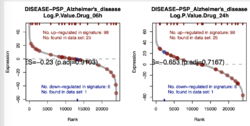
tree -L 1 ~/github/ssGSEA2.0/example/gct/2021-03-20/

├── PI3K_pert_logP_n2x23936_ssGSEA-combined.gct
├── PI3K_pert_logP_n2x23936_ssGSEA-fdr-pvalues.gct
├── PI3K_pert_logP_n2x23936_ssGSEA-pvalues.gct
├── PI3K_pert_logP_n2x23936_ssGSEA-scores.gct
├── PI3K_pert_logP_n2x23936_ssGSEA.RData
├── parameters.txt
├── rank-plots
├── run.log
└── signature_gct

tree ~/github/ssGSEA2.0/example/gct/2021-03-20/rank-plots | head -3
# 102 files. One file per matched gene set
├── DISEASE.PSP_Alzheime_2.pdf
├── DISEASE.PSP_breast_c_2.pdf

tree ~/github/ssGSEA2.0/example/gct/2021-03-20/signature_gct | head -3
# 102 files. One file per matched gene set
├── DISEASE.PSP_Alzheimer.s_disease_n2x23.gct
├── DISEASE.PSP_breast_cancer_n2x14.gct
Since the GCT file contains 2 samples (the last 2 columns), ssGSEA produces one rank plot for each gene set (with adjusted p-value & the plot could contain multiple samples). The ES scores are saved in <PI3K_pert_logP_n2x23936_ssGSEA-scores> and adjust p-values are saved in <PI3K_pert_logP_n2x23936_ssGSEA-fdr-pvalues>.
- Some possible problems using ssGSEA to replace GSEA for DE analysis? See a toy example on Single Sample GSEA (ssGSEA) and dynamic range of expression. PS: the rank values table is wrong; they should be reversed.
- In general terms, PLAGE and z-score are parametric and should perform well with close-to-Gaussian expression profiles, and ssGSEA and GSVA are non-parametric and more robust to departures of Gaussianity in gene expression data. See Method and kcdf arguments in gsva package
- Some discussions from biostars.org. Find -> "ssgsea"
- Some papers.
- 【生信分析 3】教你看懂GSEA和ssGSEA分析结果. No groups/classes in the data (6:33). Output is a heatmap. Each value is computed sample by sample. Rows = gene set. Columns = (sorted by the 1st gene set) samples.
- Gene set analysis: GSVA, Z-Score, and fold-changes

escape
escape - Easy single cell analysis platform for enrichment. Github.
sTAM
- Paper sTAM: An Online Tool for the Discovery of miRNA-Set Level Disease Biomarkers 2020
- http://mir.rnanut.net/stam. It performs single-sample miRNA-set enrichment analysis (ssMSEA) to help identify disease-related biomarkers.
VIPER + RNAseq
- Conceptually similar to GSEA or KSEA, but VIPER focuses on transcription factors.
- VIPER = Virtual Inference of Protein-activity by Enriched Regulon analysis
- Input is Gene expression + regulon, i.e., the set of genes regulated by each TF (with weights/interaction signs).
- Output:
- Activity score for each TF/regulator.
- Optional significance estimates via permutations or bootstrapping.
- Network-based inference of protein activity helps functionalize the genetic landscape of cancer
- viper R package from Bioconductor.
- msviper() is for multiple sample version
- viper() is for single sample
data(bcellViper, package="bcellViper")
d1 <- exprs(dset) # 6249 x 211
res <- viper(d1, regulon) # 621 x 211

regulon
# Object of class regulon with 621 regulators, 6249 targets and 172240 interactions

summary(c(d1))
#    Min. 1st Qu.  Median    Mean 3rd Qu.    Max.
#  -9.057   6.972   8.688   8.349  10.038  16.071
res[1:2, 1:5]
#      GSM44075 GSM44078 GSM44080 GSM44081 GSM44082
# AATF 7.182338 4.642805 7.485831 7.083181 6.473570
# ADNP 3.459128 1.972037 3.362503 4.690003 3.415285
621 regulators → These are the proteins (mostly TFs) whose activity VIPER can infer. Each regulator has a set of target genes.
6249 targets → The genes whose expression is controlled by these regulators.
172,240 interactions → Each interaction links a regulator to a target gene, with information about the mode of regulation (tfmode: activating/repressing) and likelihood/weight (confidence of interaction).
- Generate a regulon using ARACNe
- ARACNe (Algorithm for the Reconstruction of Accurate Cellular Networks) is commonly used to reverse-engineer transcriptional regulatory networks from gene expression data.
- Steps:
- Input a gene expression matrix.
- Run ARACNe to infer regulator → target interactions.
- Convert ARACNe output to VIPER-compatible regulon using aracne2regulon():
regulon <- aracne2regulon(aracneOutput, expr)
- Comparison
Algorithm Input data Target type Analogy GSEA RNA expression Pathway genes "Pathway enrichment" VIPER RNA expression TF targets (regulons) "TF activity enrichment" KSEA Phosphoproteomics Kinase substrates "Kinase activity enrichment"
KSEA and protein
- https://github.com/casecpb/KSEA and the paper The KSEA App: a web-based tool for kinase activity inference from quantitative phosphoproteomics
- In KSEA, the analysis focuses on kinase substrate gene sets, which are predefined groups of individual substrate genes known to be phosphorylated by a specific kinase. The algorithm assesses whether these sets of substrate genes are enriched at the top or bottom of a ranked list based on gene expression (or sometimes phosphorylation) changes.
- A kinase is a type of protein that acts like a little worker whose main job is to attach a special tag (a phosphate group) to other proteins.
- This tagging process is called phosphorylation, and it's a very common way for cells to control how other proteins work. By adding this tag, a kinase can switch a protein "on" or "off," change its shape, or tell it to interact with other molecules.
- Different kinases control different sets of protein "switches." This allows the cell to respond to signals from its environment and regulate all sorts of processes, from growth and movement to how it uses energy.
- In GSEA, the analysis focuses on gene sets, which are predefined groups of individual genes that share a common biological function, pathway, or chromosomal location. The algorithm assesses whether these sets of genes are enriched at the top or bottom of a ranked list based on gene expression changes.
- Comparison of KSEA to GSEA
Comparison of KSEA and GSEA Feature KSEA (Kinase Set Enrichment Analysis) GSEA (Gene Set Enrichment Analysis) Focus Enrichment of kinase substrate gene sets. Identifies kinases with altered activity. Enrichment of gene sets. Identifies pathways, biological processes, or genomic regions with altered expression. Input Data Typically gene expression data (e.g., microarray, RNA-seq) and a database of known kinase-substrate relationships. Typically gene expression data (e.g., microarray, RNA-seq) and a predefined gene set database (e.g., GO, KEGG, MSigDB). Analysis Goal To infer upstream regulatory kinases that are likely responsible for observed gene expression changes. To determine whether a priori defined sets of genes show statistically significant, concordant differences between two biological states. Mechanism Ranks genes based on expression changes and then assesses whether the substrates of specific kinases are over-represented at the top or bottom of the ranked list. Ranks genes based on expression changes and then assesses whether the genes within a defined set are non-randomly distributed towards the top or bottom of the ranked list. Output A ranked list of kinases, indicating their potential involvement in the observed expression changes, along with enrichment scores and p-values. A ranked list of gene sets, indicating their enrichment in the experimental conditions, along with enrichment scores and p-values. Biological Insight Provides insights into signaling pathways and upstream regulatory mechanisms involving kinases. Provides insights into affected biological pathways, processes, and functional categories. Data Requirements Requires knowledge of kinase-substrate interactions, which might be less comprehensive than general gene set databases. Relies on well-annotated and comprehensive gene set databases.
KSEA input
| Protein | Gene | Peptide | Residue.Both | p | FC |
|---|---|---|---|---|---|
| P31749 | AKT1 | AASTVEpSPK | S473 | 0.324 | 1.5 |
| Q9Y243 | GSK3B | GSRLpSPVRA | S9 | 0.258 | -0.7 |
- "Residue.Both": Site of phosphorylation (e.g., S473, T308). (S = Serine, 473 = position). You can also have multiple sites per protein (e.g., T308;S473). S = Serine, T = Threonine, Y = Tyrosine. A residue is just a fancy term for an amino acid within a protein or peptide chain.
- p: the p-value of the differential phosphorylation between the two groups
- FC: the fold change between the two groups’ peptide intensities (not log-transformed);
Question: The number of kinases that the KSEA App considers depends on the kinase–substrate database it utilizes
- Initially, using only curated data from PhosphoSitePlus (PSP), the app could score approximately 175 kinases.
- However, by incorporating predicted kinase–substrate relationships from NetworKIN, this number increases to about 235 kinases
- It's important to note that the actual number of kinases scored in your analysis will depend on the overlap between your phosphoproteomics data and the kinase–substrate database used. If your dataset includes phosphorylation sites that match the substrates in the database, the corresponding kinases can be evaluated for activity.
Benchmarking
- Benchmarking substrate-based kinase activity inference using phosphoproteomic data
- Comprehensive evaluation of phosphoproteomic-based kinase activity inference 2025 & the benchmarKIN package.
- The study found that while most computational methods performed similarly, the choice of kinase-substrate library significantly impacted the inferred activities. Combining manually curated libraries, such as PhosphoSitePlus, PTMsigDB, and GPS gold, demonstrated superior performance in recapitulating kinase activities. Additionally, incorporating predicted targets from NetworKIN further enhanced performance in the tumor-based evaluation.
Benchmark
Toward a gold standard for benchmarking gene set enrichment analysis Geistlinger, 2021. GSEABenchmarkeR package in Bioconductor.
phantasus
- phantasus Visual and interactive gene expression analysis. read.gct(), write.gct(), getGSE(), loadGEO(), gseaPlot().
- Using Phantasus application
PhenoExam
PhenoExam: gene set analyses through integration of different phenotype databa
Selected papers
- On the influence of several factors on pathway enrichment analysis Mubeen 2022
- Popularity and performance of bioinformatics software: the case of gene set analysis Xie 2021
- Gene set analysis approaches for RNA-seq data: performance evaluation and application guideline Rahmatallah 2015. Simulated RNA-Seq data was considered too.
- Gene set analysis methods: a systematic comparison Mathur, 2018
- A Comparison of Gene Set Analysis Methods in Terms of Sensitivity, Prioritization and Specificity Tarca 2013
Malacards
- MalaCards - human disease database. Paper 2018
- GSEABenchmarkeR package used it.
- (Not Malacards) KEGGandMetacoreDzPathwaysGEO Disease Datasets from GEO. This is a collection of 18 data sets for which the phenotype is a disease with a corresponding pathway in either KEGG or metacore database.This collection of datasets were used as gold standard in comparing gene set analysis methods.
- 生信数据库之疾病数据库
GSDA
Gene-set distance analysis (GSDA): a powerful tool for gene-set association analysis
Genekitr
https://github.com/GangLiLab/genekitr. twitter
KEGG
KEGGREST
- R: keggList(), keggGet()
install.packages("BiocManager")
BiocManager::install("KEGGREST")

packageVersion("KEGGREST") # [1] ‘1.38.0’
library(KEGGREST)

# Step 1: Get a list of KEGG pathways for Homo sapiens
kegg_pathways <- keggList("pathway", "hsa")  # "hsa" = Homo sapiens

# Step 2: Function to extract gene symbols from a KEGG pathway
get_kegg_genes <- function(pathway_id) {
  # Get pathway details
  pathway_info <- keggGet(pathway_id)

  if (length(pathway_info) == 0 || is.null(pathway_info[[1]]$GENE)) {
    return(NULL)  # Skip pathways with no gene information
  }

  # Extract gene entries (alternating gene IDs and descriptions)
  gene_entries <- pathway_info[[1]]$GENE

  # Every even-indexed element corresponds to a gene symbol
  raw_gene_symbols <- gene_entries[seq(2, length(gene_entries), by = 2)]

  # Extract part before the semicolon using sub() function
  gene_symbols <- sub(";.*", "", raw_gene_symbols)

  return(gene_symbols)
}

# Step 3: Extract gene sets for each pathway
# kegg_gene_sets <- lapply(names(kegg_pathways), get_kegg_genes)
kegg_gene_sets <- list()
for (pathway_id in names(kegg_pathways)) {
  kegg_gene_sets[[pathway_id]] <- get_kegg_genes(pathway_id)
}

# Step 5: Remove NULL entries (pathways without genes)
kegg_gene_sets <- kegg_gene_sets[!sapply(kegg_gene_sets, is.null)]
length(kegg_gene_sets) # [1] 351

# Verify: https://www.genome.jp/dbget-bin/www_bget?pathway:hsa00220
kegg_gene_sets[["hsa00220"]]
# [1] "OTC"          "ASS1"         "ASL"          "ARG1"         "ARG2"
# [6] "NOS1"         "NOS2"         "NOS3"         "GLS2"         "GLS"
# [11] "GLUL"         "CAD"          "CPS1"         "GLUD1"        "GLUD2"
# [16] "GOT1L1"       "GOT1"         "GOT2"         "GPT"          "GPT2"
# [21] "NAGS"         "ABHD14A-ACY1" "ACY1"

cat(keggInfo("kegg"))
# kegg             Kyoto Encyclopedia of Genes and Genomes
# kegg             Release 110.0+/06-12, Jun 24
#                  Kanehisa Laboratories
#                  pathway   1,189,366 entries
#                  brite       391,405 entries
#                  module          561 entries
#                  orthology    26,801 entries
#                  genome       24,756 entries
#                  genes     54,580,049 entries
#                  compound     19,356 entries
#                  glycan       11,220 entries
#                  reaction     12,089 entries
#                  rclass        3,194 entries
#                  enzyme        8,158 entries
#                  network       1,549 entries
#                  variant       1,452 entries
#                  disease       2,754 entries
#                  drug         12,455 entries
#                  dgroup        2,473 entries
It seems there is no way to do query based on a specific date/release. So we need to save the objects
# Save the data and metadata
saveRDS(pathways, file = "hsa_pathways.rds")
saveRDS(pathway_info, file = paste0(pathway_id, "_info.rds"))
- Download a pathway in KGML or other formats. For example, hsa00220.
- KGML (KEGG Markup Language) is an XML-based format used by the KEGG (Kyoto Encyclopedia of Genes and Genomes) database to represent pathway maps.
png <- keggGet("hsa00220", "image") ## retrieves the image file of a
                                    ## pathway map
t <- tempfile()
t <- paste0(t, ".png")
library(png)
writePNG(png, t)

res <- keggGet("hsa00220", "kgml")
str(res)
- A KGML file typically contains the following components:
- Pathway: The root element that includes general information about the pathway, such as its name, organism, and version.
- Entry: Represents entities such as genes, proteins, compounds, and groups within the pathway.
- Relation: Describes the interactions between entities, including regulatory relationships.
- Reaction: Details the biochemical reactions, including substrates, products, and enzymes involved.
- Tools Supporting KGML:
- KEGG Mapper
- Cytoscape
- PathVisio
- keggList(). It returns 359 KEGG pathways and 19356 compounds as of now (6/12/2024).
pathways <- keggList("pathway", "hsa") length(pathways) # [1] 359 str(pathways) # Named chr [1:359] "Metabolic pathways - Homo sapiens (human)" ... # - attr(*, "names")= chr [1:359] "hsa01100" "hsa01200" "hsa01210" "hsa01212" ... Download all KEGG pathway compounds keggList("compound") |> length() # [1] 19356 keggList("compound") |> names() |> head() # [1] "C00001" "C00002" "C00003" "C00004" "C00005" "C00006" - keggLink(). It returns 8840 NCBI genes, 359 KEGG pathways, and 1444 unique Enzymes.
help
# keggLink(target_database, source_database) entrez2path <- keggLink("pathway", "hsa") ## KEGG pathways linked from each of the human genes ## equivalent to 'get.genes.by.pathway' in KEGGSOAP length(entrez2path) # [1] 37310 length(unique(names(entrez2path))) # [1] 8840 length(unique(entrez2path)) # [1] 359 path2entrez <- keggLink("hsa", "pathway") ## human genes linked from each of the KEGG pathways ## equivalent to 'get.pathways.by.genes' in KEGGSOAP length(path2entrez) # [1] 37310 length(unique(path2entrez)) # [1] 8840 keggLink("pathway", c("hsa:10458", "ece:Z5100")) ## KEGG pathways linked from a ## human gene and an E. coli ## O157 gene keggLink("hsa:126") entrez2ec <- keggLink("enzyme", "hsa") # return pairs of human gene IDs and their associated enzyme EC numbers. length(entrez2ec) # [1] 3832 entrez2ec[1:2] # One gene ID can correspond to multiple enzymes. Similarly, vice versa. # hsa:9344 hsa:5894 # "ec:2.7.11.1" "ec:2.7.11.1" length(unique(names(entrez2ec))) # [1] 3493 length(unique(entrez2ec)) # [1] 1444 - keggGet(). https://www.genecards.org/cgi-bin/carddisp.pl?gene=TAOK2
gene_info <- keggGet("hsa:9344") # 9344 is NCBI gene ID print(gene_info) names(gene_info[[1]]) # [1] "ENTRY" "SYMBOL" "NAME" "ORTHOLOGY" "ORGANISM" "PATHWAY" # [7] "NETWORK" "DISEASE" "BRITE" "POSITION" "MOTIF" "DBLINKS" # [13] "STRUCTURE" "AASEQ" "NTSEQ" gene_info[[1]]$NAME # [1] "(RefSeq) TAO kinase 2" gene_info[[1]]$SYMBOL # Primary + aliases # [1] "TAOK2, MAP3K17, PSK, PSK1, PSK1-BETA, TAO1, TAO2, Tao2beta" enzyme_info <- keggGet("ec:2.7.11.1") str(enzyme_info) names(enzyme_info[[1]]) # [1] "ENTRY" "NAME" "CLASS" "REACTION" "COMMENT" "HISTORY" # [7] "ORTHOLOGY" "GENES" "DBLINKS" "REFERENCE" - listDatabases()
listDatabases()
 [1] "pathway"  "brite"    "module"   "ko"       "genome"   "vg"       "ag"
 [8] "compound" "glycan"   "reaction" "rclass"   "enzyme"   "disease"  "drug"
[15] "dgroup"   "environ"  "genes"    "ligand"   "kegg"
- keggCompounds()
- keggInfo()
- keggFind()
- keggConv()
MSigDB
https://www.gsea-msigdb.org/gsea/msigdb/
- C1: Hallmark
- C2: Curated gene sets including BioCarta, KEGG, Reactome
- C5: Oncology
Hallmark
- HALLMARK_EPITHELIAL_MESENCHYMAL_TRANSITION/EMT from MsigDB
- Epithelial and mesenchymal gene signatures. See here. I save the gene lists in Github.
- 'Table S1A. Generic EMT signature for tumour ' is really more interesting since Epi is more tumor related. The first 145 are epi, the rest (315-145=170) are mes.
- Epithelial (170 genes), mesenchymal gene signatures 218-170=48 genes). Tan et al. 2014 and can be found in the 'Table S1B. Generic EMT signature for cell line ’.
RaMP
- https://rampdb.nih.gov/, https://rampdb.nih.gov/pathways-from-analytes
- https://github.com/ncats/RaMP-DB
igraph
- igraph from CRAN: Network Analysis and Visualization. It can handle large graphs very well and provides functions for generating random and regular graphs, graph visualization, centrality methods and much more.
- Integration: Works well within the R ecosystem and can be easily combined with other R packages for data manipulation (e.g., dplyr) and visualization (e.g., ggplot2).
- Applications:
- It can be used with the plotly or networkD3 package to create interactive network.
Rgraphviz
- Rgraphviz from Bioconductor
- Integration: Primarily integrates with Graphviz and the Bioconductor ecosystem. It is often used in bioinformatics for visualizing biological networks like protein-protein interactions or metabolic pathways.
- Dependency: Requires Graphviz to be installed separately, which can add complexity to setup and usage.
- Applications:
- It can be used with the visNetwork package (using vis.js javascript library) to create interactive network visualizations.