Regression
Linear Regression
- Regression Models for Data Science in R by Brian Caffo
- Regression and Other Stories (book) by Andrew Gelman, Jennifer Hill, Aki Vehtari
Comic
MSE
- Mean squared error (within-sample)
- Mean squared prediction error (out-of-sample)
- Is MSE decreasing with increasing number of explanatory variables?
- Calculate (Root) Mean Squared Error in R (5 Examples)
Coefficient of determination R2
- Relationship in the simple linear regression (intercept is included)

- https://en.wikipedia.org/wiki/Coefficient_of_determination.
- R2 is expressed as the ratio of the explained variance to the total variance.
- It is a statistical measure of how well the regression predictions approximate the real data points.
- See the wikipedia page for a list of caveats of R2 including correlation does not imply causation.
- Based on the data collected, my tennis ball will reach orbit by tomorrow. R2=0.85 in the following example.

- Avoid R-squared to judge regression model performance
- R2 = RSS/TSS (model based)
- R2(x~y) = R2(y~x)
- R2 = Pearson correlation^2 (not model based)
- summary(lm())$r.squared. See Extract R-square value with R in linear models
- How to interpret root mean squared error (RMSE) vs standard deviation? 𝑅2 value.
- coefficient of determination R^2 (can be negative?)
- The R-squared and nonlinear regression: a difficult marriage?
- How R2 and RMSE are calculated in cross-validation of pls R
- How to Interpret R Squared and Goodness of Fit in Regression Analysis
- Limitations of R-squared: R-squared does not inform if the regression model has an adequate fit or not. It can be arbitrarily low when the model is completely correct. See How to make R-squared useless.
- Low R-squared and High R-squared values. A regression model with high R2 value can lead to – as the statisticians call it – specification bias. See an example.
- Five Reasons Why Your R-squared can be Too High
- R-squared is a biased estimate. R-squared estimates tend to be greater than the correct population value.
- Overfitting your model. This problem occurs when the model is too complex.
library(ggplot2)
set.seed(123)
x <- 1:100
y <- x + rnorm(100, sd = 10)
model1 <- lm(y ~ x)
summary(model1)$r.squared  # 0.914

# Now, let's add some noise variables
noise <- matrix(rnorm(100*1000), ncol = 1000)
model2 <- lm(y ~ x + noise)
summary(model2)$r.squared  # 1
- Data mining and chance correlations. Multiple hypotheses.
- Trends in Panel (Time Series) Data
- Form of a Variable - include a different form of the same variable for both the dependent variable and an independent variable.
- Relationship between R squared and Pearson correlation coefficient
- What is the difference between Pearson R and Simple Linear Regression?
- R2 and MSE
- [math]\displaystyle{ \begin{align} R^2 &= 1 - \frac{SSE}{SST} \\ &= 1 - \frac{MSE}{Var(y)} \end{align} }[/math]
- lasso/glmnet
- Beware of R2: simple, unambiguous assessment of the prediction accuracy of QSAR and QSPR models Alexander 2015. Golbraikh and Tropsha which identified the inadequacy of the leave-one-out cross-validation R2 (denoted as q2 in this case) calculated on training set data as a reliable characteristic of the model predictivity.
- The R-squared and nonlinear regression: a difficult marriage?
Pearson correlation and linear regression slope
- Simple Linear Regression and Correlation
- Pearson Correlation and Linear Regression, Comparing Correlation and Slope
- [math]\displaystyle{ \begin{align} b_1 &= r \frac{S_y}{S_x} \end{align} }[/math]
where [math]\displaystyle{ S_x=\sqrt{\sum(x-\bar{x})^2} }[/math].
set.seed(1)
x <- rnorm(10); y <-rnorm(10)
coef(lm(y~x))
# (Intercept)           x
#   0.3170798  -0.5161377

cor(x, y)*sd(y)/sd(x)
# [1] -0.5161377
Different models (in R)
http://www.quantide.com/raccoon-ch-1-introduction-to-linear-models-with-r/
Factor Variables
Regression With Factor Variables
dummy.coef.lm() in R
Extracts coefficients in terms of the original levels of the coefficients rather than the coded variables.
Signif. codes/asterisks
Signif. codes: 0 '***' 0.001 '**' 0.01 '*' 0.05 '.' 0.1 ' ' 1
Add Regression Line per Group to Scatterplot
How To Add Regression Line per Group to Scatterplot in ggplot2?
penguins_df %>%
  ggplot(aes(x=culmen_length_mm,
             y=flipper_length_mm,
             color=species))+
  geom_point()+
  geom_smooth(method="lm", se = FALSE)
model.matrix, design matrix
- https://en.wikipedia.org/wiki/Design_matrix
- ExploreModelMatrix: Explore design matrices interactively with R/Shiny. Paper on F1000research.
- model(~A+B) will return 1 + (a-1) + (b-1) columns. See an example Batch effects and confounders.
Contrasts in linear regression
- Page 147 of Modern Applied Statistics with S (4th ed)
- https://biologyforfun.wordpress.com/2015/01/13/using-and-interpreting-different-contrasts-in-linear-models-in-r/ This explains the meanings of 'treatment', 'helmert' and 'sum' contrasts.
- A (sort of) Complete Guide to Contrasts in R by Rose Maier
mat

##      constant NLvMH  NvL  MvH
## [1,]        1  -0.5  0.5  0.0
## [2,]        1  -0.5 -0.5  0.0
## [3,]        1   0.5  0.0  0.5
## [4,]        1   0.5  0.0 -0.5
mat <- mat[ , -1]

model7 <- lm(y ~ dose, data=data, contrasts=list(dose=mat) )
summary(model7)

## Coefficients:
##             Estimate Std. Error t value Pr(>|t|)
## (Intercept)  118.578      1.076 110.187  < 2e-16 ***
## doseNLvMH      3.179      2.152   1.477  0.14215
## doseNvL       -8.723      3.044  -2.866  0.00489 **
## doseMvH       13.232      3.044   4.347 2.84e-05 ***

# double check your contrasts
attributes(model7$qr$qr)$contrasts
## $dose
##      NLvMH  NvL  MvH
## None  -0.5  0.5  0.0
## Low   -0.5 -0.5  0.0
## Med    0.5  0.0  0.5
## High   0.5  0.0 -0.5

library(dplyr)
dose.means <- summarize(group_by(data, dose), y.mean=mean(y))
dose.means
## Source: local data frame [4 x 2]
##
##   dose   y.mean
## 1 None 112.6267
## 2  Low 121.3500
## 3  Med 126.7839
## 4 High 113.5517

# The coefficient estimate for the first contrast (3.18) equals the average of
# the last two groups (126.78 + 113.55 /2 = 120.17) minus the average of
# the first two groups (112.63 + 121.35 /2 = 116.99).
Multicollinearity
- A toy example
n <- 100
set.seed(1)
x1 <- rnorm(n)
e <- rnorm(n)*.01
y <- x1 + e
cor(y, e)  # 0.00966967
cor(y, x1) # 0.9999
lm(y ~ x1) |> summary()      # p<2e-16

set.seed(2)
x2 <- x1 + rnorm(n)*.1       # x2 = x1 + noise
cor(x1, x2)  # .99
lm(y ~ x1 + x2) |> summary() # x2 insig
lm(y~ x2) |> summary()       # x2 sig

set.seed(3)
x3 <- x1 + rnorm(n)*.0001    # x3 = x1 + tiny noise
cor(x1, x3) # 1
lm(y ~ x1 + x3) |> summary() # both insig. SURPRISE!
lm(y ~ x1) |> summary()

x4 <- x1                     # x4 is exactly equal to x1
lm(y~ x1 + x4) |> summary()  # x4 coef not defined because of singularities
lm(y~ x4 + x1) |> summary()  # x1 coef not defined because of singularities
Consider lasso
fit <- cv.glmnet(x=cbind(x1, x3, matrix(rnorm(n*10), nr=n)), y=y)
coefficients(fit, s = "lambda.min")
# 13 x 1 sparse Matrix of class "dgCMatrix"
#                      s1
# (Intercept) 0.002797165
# x1          0.970839175
# x3          .
#             .

fit <- cv.glmnet(x=cbind(x1, x4, matrix(rnorm(n*10), nr=n)), y=y)
coefficients(fit, s = "lambda.min")
# 13 x 1 sparse Matrix of class "dgCMatrix"
#                       s1
# (Intercept) 2.797165e-03
# x1          9.708392e-01
# x4          6.939215e-18
#             .

fit <- cv.glmnet(x=cbind(x4, x1, matrix(rnorm(n*10), nr=n)), y=y)
coefficients(fit, s = "lambda.min")
# 13 x 1 sparse Matrix of class "dgCMatrix"
#                      s1
# (Intercept) 2.797165e-03
# x4          9.708392e-01
# x1          6.93 9215e-18
#             .
- How to Fix in R: not defined because of singularities
- Multicollinearity in R
- Detecting multicollinearity — it’s not that easy sometimes
- alias: Find Aliases (Dependencies) In A Model
> op <- options(contrasts = c("contr.helmert", "contr.poly"))
> npk.aov <- aov(yield ~ block + N*P*K, npk)
> alias(npk.aov)
Model :
yield ~ block + N * P * K

Complete :
         (Intercept) block1 block2 block3 block4 block5 N1    P1    K1    N1:P1 N1:K1 P1:K1
N1:P1:K1     0           1    1/3    1/6  -3/10   -1/5      0     0     0     0     0     0

> options(op)
Exposure
https://en.mimi.hu/mathematics/exposure_variable.html
Independent variable = predictor = explanatory = exposure variable
Marginal effects
- CRAN, https://marginaleffects.com/
- The marginaleffects package for R. Compute and plot adjusted predictions, contrasts, marginal effects, and marginal means for 69 classes of statistical models in R. Conduct linear and non-linear hypothesis tests using the delta method.
- Slides
Confounders, confounding
- What is a Confounding Variable? (Definition & Example). Confounding variable is a variable that can affect the relationship between the two variables under study. Requirements for Confounding Variables:
- It must be correlated with the independent variable.
- It must have a causal relationship with the dependent variable.
- Confounders Introduction to Data Science by Irizarry
- If X and Y are correlated, we call Z a confounder if changes in Z causes changes in both X and Y.
- https://en.wikipedia.org/wiki/Confounding
- A method for controlling complex confounding effects in the detection of adverse drug reactions using electronic health records. It provides a rule to identify a confounder.
- http://anythingbutrbitrary.blogspot.com/2016/01/how-to-create-confounders-with.html (R example)
- Logistic Regression: Confounding and Colinearity
- Identifying a confounder
- Using a change in a continuous explanatory variable to test changes in gene expression with limma. If the second model gives just as much DE as the first, then that is evidence that expression changes between visits are largely explained by the weight loss.
- Is it possible to have a variable that acts as both an effect modifier and a confounder?
- Which test to use to check if a possible confounder impacts a 0 / 1 result?
- Addressing confounding artifacts in reconstruction of gene co-expression networks Parsana 2019
- Up Your Steps to Lower Blood Pressure, Heart Study Suggests
- Over about five months, participants averaged roughly 7,500 steps per day. Those with a higher daily step count had significantly lower blood pressure.
- the researchers found that systolic blood pressure was about 0.45 points lower for every 1,000 daily steps taken
- The link between daily step count and blood pressure was no longer significant when body mass index (BMI) was taken into account, however.
- Empirical economics with r (part b): confounders, proxies and sources of exogenous variations, causal effects.
- No, you have not controlled for confounders
- Visual Demonstration of Residual Confounding. Don't dichotomize a continuous variable.
- See Randomized block design
- Simulating confounders, colliders and mediators
- Age is a confounder for some disease.
- Suppose X1 and X2 are predictors for Y
- What Does Confounding Mean? Confounding occurs when the association between a predictor and outcome is distorted by a third variable. More specifically, X1 and X2 are confounded with respect to Y when:
- Both X1 and X2 are associated with Y
- X1 and X2 are associated with each other
- This correlation between X1 and X2 makes it difficult to isolate the independent effect of each predictor on Y
- An example. A concrete example: Suppose you're studying the effect of coffee consumption (X1) on heart disease (Y), but coffee drinkers also tend to smoke more (X2). Smoking is associated with both coffee drinking and heart disease. If you only look at Y vs X1, you might incorrectly attribute some of smoking's effect on heart disease to coffee consumption.
- The Key Issue
- The coefficient for X1 in a simple regression (Y ~ X1) includes both its direct effect AND the indirect pathway through its association with X2
- Comparing Y ~ X1, Y ~ X2, and Y ~ X1 + X2 often reveals substantial changes in coefficients when confounding is present
- How to Test for Confounding
- Compare regression coefficients (Y~X1, Y~X2, Y~X1+X2). If coefficients for X1 or X2 change substantially when you add the other variable, confounding is likely present. A common rule of thumb is a change of >10-20% in the coefficient.
- Check correlation between predictors. Calculate the correlation between X1 and X2. High correlation (positive or negative) suggests potential confounding.
- Use variance inflation factor (VIF). VIF quantifies how much the variance of a regression coefficient is inflated due to correlation with other predictors. VIF > 5 or 10 suggests problematic confounding (multicollinearity).
- Compare R² values. If R² for Y ~ X1 + X2 is not much larger than max(R² for Y ~ X1, R² for Y ~ X2), the predictors may be explaining overlapping variance due to confounding.
- Stratified analysis. Examine the X1-Y relationship within levels of X2. If the relationship changes across strata, X2 may be confounding the X1-Y association.
- What Does Confounding Mean? Confounding occurs when the association between a predictor and outcome is distorted by a third variable. More specifically, X1 and X2 are confounded with respect to Y when:
Simulated data
Question: gene expression ~ age + condition (condition is significant) but gene expression ~ condition (condition is not significant). Releted post: Highly DE genes but small count difference within conditions.
Possible Explanation
- Confounding Variable: Age might be a confounding variable, meaning it influences both gene expression and condition. When you include age, you control for its effect, which clarifies the relationship between condition and gene expression.
- Interaction Effect: There might be an interaction between age and condition. In the full model, the combined effect of age and condition provides a clearer picture of how condition affects gene expression.
- Multicollinearity: It could also indicate multicollinearity, where age and condition are correlated. Including both variables might change the significance levels.
Simulated data
- Confounding only (covariates).
# Simulate data
n <- 100
age <- rnorm(n, mean = 50, sd = 10)  # Continuous variable for age

# Influence condition by age: older individuals more likely to have condition
condition <- ifelse(age > 50, 1, 0)

# Simulate gene expression with confounding but no interaction or multicollinearity
expression <- 5 + 0.3*age + 2*condition + rnorm(n)

# Create data frame
df <- data.frame(age, condition, expression)
- Interaction only
# Set seed for reproducibility
set.seed(123)

# Simulate data
n <- 100
age <- rnorm(n, mean = 50, sd = 10)  # Continuous variable for age
condition <- rbinom(n, 1, 0.5)       # Binary variable for condition

# Simulate gene expression with interaction, no confounding, no multicollinearity
expression <- 5 + 0.3*age + 2*condition + 0.5*age*condition + rnorm(n)

# Create data frame
df <- data.frame(age, condition, expression)
- multicollinearity only (covariates)
# Set seed for reproducibility
set.seed(123)

# Simulate data
n <- 100
age <- rnorm(n, mean = 50, sd = 10)  # Continuous variable for age
# Create a multicollinear variable that is highly correlated with age
age_collinear <- age + rnorm(n, mean = 0, sd = 2)

# Binary condition variable, independent of age
condition <- rbinom(n, 1, 0.5)

# Simulate gene expression with no confounding or interaction but with multicollinearity
expression <- 5 + 0.3*age + 0.3*age_collinear + 2*condition + rnorm(n)

# Create data frame
df <- data.frame(age, age_collinear, condition, expression)

# Check multicollinearity
library(car)
vif(lm(expression ~ age + age_collinear + condition, data = df))
# A VIF value above 10 generally indicates high multicollinearity,
# but even values above 5 might be concerning.
- Everything
# Load necessary library
library(dplyr)

# Set seed for reproducibility
set.seed(123)

# Simulate data
n <- 100
age <- rnorm(n, mean = 50, sd = 10)  # Continuous variable for age
# Influence condition by age: older individuals more likely to have condition
condition <- ifelse(age > 50, 1, 0)

# Create a multicollinear variable that is highly correlated with age
age_collinear <- age + rnorm(n, mean = 0, sd = 2)

# Simulate gene expression with confounding, multicollinearity, and interaction
expression <- 5 + 0.3*age + 0.3*age_collinear + 2*condition + 0.5*age*condition + rnorm(n)

# Create data frame
df <- data.frame(age, age_collinear, condition, expression)

# Summary of data
summary(df)

# Check multicollinearity
library(car)
vif(lm(expression ~ age + age_collinear + condition, data = df))
Plotting
- Stratified Scatter Plot
plot(df$age, df$expression, col=as.factor(df$condition), pch=16, main="Stratified Plot: Age vs. Expression by Condition", xlab="Age", ylab="Gene Expression") legend("topright", legend=levels(as.factor(df$condition)), col=1:length(levels(as.factor(df$condition))), pch=16) - Pair Plot
pairs(~expression + age + condition, data=df,
      main="Pair Plot: Expression, Age, Condition",
      col=as.factor(df$condition), pch=16)
Confidence interval vs prediction interval
Confidence intervals tell you about how well you have determined the mean E(Y). Prediction intervals tell you where you can expect to see the next data point sampled. That is, CI is computed using Var(E(Y|X)) and PI is computed using Var(E(Y|X) + e).
- http://www.graphpad.com/support/faqid/1506/
- http://en.wikipedia.org/wiki/Prediction_interval
- http://robjhyndman.com/hyndsight/intervals/
- https://stat.duke.edu/courses/Fall13/sta101/slides/unit7lec3H.pdf
- https://datascienceplus.com/prediction-interval-the-wider-sister-of-confidence-interval/
- Confidence and prediction intervals explained... (with a Shiny app!)
Homoscedasticity, Heteroskedasticity, Check model for (non-)constant error variance
- Dealing with heteroskedasticity; regression with robust standard errors using R
- performance package check_heteroscedasticity(x, ...) and check_heteroskedasticity(x, ...)
- easystats: Quickly investigate model performance
- Homoscedasticity in Regression Analysis
- Exploring Variance Inflation Factor (VIF) in R: A Practical Guide.
Linear regression with Map Reduce
https://freakonometrics.hypotheses.org/53269
Relationship between multiple variables
Visualizing the relationship between multiple variables
Model fitting evaluation, Q-Q plot
Added variable plots
Added Variable Plots/partial-regression plots
Generalized least squares
- gls from the nlme package. The errors are allowed to be correlated and/or have unequal variances.
- varClasses: varPower(), varExp(), varConstPower(), varFunc()
- summary()$varBeta (variance of coefficient estimates), summary()$sigma (error sigma)
- intervals()$coef (coefficient estimates), intervals()$varStruct (lower, est, upper of variance function)
- anova()
- 95 Prediction intervals: predict(gls, newdata, interval = "prediction", level = .95) OR predict(gls, newdata) +/ qt(0.975,n-2)*se*sqrt(1+1/n+xd/ssx) where se=sigma.param*newx^pow.param, xd=(newx-xbar)^2, pow.param = coef(glsOjb$modelStruct$varStruct).
- gls() vs. lme() in the nlme package
- How to use Generalized Least Square gls() in r. Chapter 5.2.1 (page 208) in Mixed Effects Models in S and S-Plus by Pinheiro and Bates 2000.
- https://asancpt.github.io/nlme/chapter-8.html
- The lme function by Peter Dalgaard
- http://halweb.uc3m.es/esp/Personal/personas/durban/esp/web/notes/gls.pdf
Reduced rank regression
- The book Multivariate Reduced-Rank Regression by Velu, Raja & Reinsel, Gregory C.
- Generalized Low Rank Models (GLRM) and h2o
Singular value decomposition
- MATRIX DECOMPOSITIONS - a shiny app
- Application to rank-k approximation of X, missing data imputation, relationship to PCA, relationship to eigen value decomposition, check multicollinearity, Moore-Penrose pseudoinverse, relationship to NMF, calculation of SVD by hand.
- https://en.wikipedia.org/wiki/Singular_value_decomposition
- Minimum norm least-squares solution to linear equation from mathworks. Solve linear equations with infinite solutions. Underdetermined system (there are fewer equations than unknowns e.g. [math]\displaystyle{ 2x_1 +3x_2 =8 }[/math]. n=1, p=2). The geometry illustration of the problem is useful. The page also provides two ways to find the solution: one is by complete orthogonal decomposition (COD) and the other is by SVD/Moore-Penrose pseudoinverse.
- Moore-Penrose matrix inverse in R
> a = matrix(c(2, 3), nr=1)
> MASS::ginv(a) * 8
         [,1]
[1,] 1.230769
[2,] 1.846154
# Same solution as matlab lsqminnorm(A,b)

> a %*% MASS::ginv(a)
     [,1]
[1,]    1
> a %*% MASS::ginv(a) %*% a
     [,1] [,2]
[1,]    2    3
> MASS::ginv   # view the source code
- Minimal Norm Solution to the least squares problem.
- The Moore-Penrose Inverse and Least Squares
- Why does SVD provide the least squares and least norm solution to 𝐴𝑥=𝑏?
Mahalanobis distance and outliers detection
- The Mahalanobis distance is a measure of the distance between a point P and a distribution D
- It is a multi-dimensional generalization of the idea of measuring how many standard deviations away P is from the mean of D.
- The Mahalanobis distance is thus unitless and scale-invariant, and takes into account the correlations of the data set.
- Distance is not always what it seems
performance::check_outliers() Outliers detection (check for influential observations)
How to Calculate Mahalanobis Distance in R
set.seed(1234)
x <- matrix(rnorm(200), nc=10)
x0 <- rnorm(10)
mu <- colMeans(x)
mahalanobis(x0, colMeans(x), var(x)) # 17.76527
t(x0-mu) %*% MASS::ginv(var(x)) %*% (x0-mu) # 17.76527

# Variance is not full rank
x <- matrix(rnorm(200), nc=20)
x0 <- rnorm(20)
mu <- colMeans(x)
t(x0-mu) %*% MASS::ginv(var(x)) %*% (x0-mu)
mahalanobis(x0, colMeans(x), var(x))
# Error in solve.default(cov, ...) :
#   system is computationally singular: reciprocal condition number = 1.93998e-19
Type 1 error
Linear Regression And Type I Error
More Data Can Hurt for Linear Regression
Estimating Coefficients for Variables in R
Trying to Trick Linear Regression - Estimating Coefficients for Variables in R
Interaction term
- how to interpret the interaction term in lm formula in R? If both x1 and x2 are numerical, then x1:x2 is actually x1*x2 in computation. That is y ~ x1 + x2 + x1:x2 is equivalent to y ~ x1 + x2 + x3 where x3 = x1*x2. The cross is literally the two terms multiplied -- interpretation will largely depend on whether var1 and var2 are both continuous (quite hard to interpret, in my opinion) or whether one of these is e.g. binary categorical (easier to consider.)
- The marginality principle revisited: Should “higher-order” terms always be accompanied by “lower-order” terms in regression analyses? 2023
Without intercept
lm(formula = y ~ x1 + x2 -1)
# or
lm(formula = y ~ x1 + x2 +0)
Intercept only model and cross-validation
n <- 20
set.seed(1)
x <- rnorm(n)
y <- 2*x + .5*rnorm(n)
plot(x, y)
df <- data.frame(x=x, y=y)
pred <- double(n)
for(i in 1:n) {
  fit <- lm(y ~ 1, data = df[-i, ])
  pred[i] <- predict(fit, df[i, ])
}
plot(y, pred)
cor(y, pred) # -1
How about 1000 simulated data?
foo <- function(n=3, debug=F) {
  x <- rnorm(n)
  y <- 2*x + .5*rnorm(n)
  df <- data.frame(x=x, y=y)
  pred <- double(n)
  for(i in 1:n) {
    fit <- lm(y ~ 1, data = df[-i, ])
    pred[i] <- predict(fit, df[i, ])
  }
  if (debug) {
    cat("num=", n*sum(y*pred)-sum(pred)*sum(y), "\n")
    cat("denom=", sqrt(n*sum(y**2) - sum(y)^2)*sqrt(n*sum(pred**2)-sum(pred)^2), "\n")
    invisible(list(y=y, pred=pred, cor=cor(y, pred)))
  } else {
    cor(y, pred)
  }
}

o <- replicate(1000, foo(n=10))
range(o) # [1] -1 -1
all.equal(o, rep(-1, 1000)) # TRUE
Note the property will not happen in k-fold CV (not LOOCV)
n <- 20; nfold <- 5
set.seed(1)
x <- rnorm(n)
y <- 2*x + .5*rnorm(n)
#plot(x, y)
df <- data.frame(x=x, y=y)
set.seed(1)
folds <- split(sample(1:n), rep(1:nfold, length = n))
pred <- double(n)
for(i in 1:nfold) {
  fit <- lm(y ~ 1, data = df[-folds[[i]], ])
  pred[folds[[i]]] <- predict(fit, df[folds[[i]], ])
}
plot(y, pred)
cor(y, pred) # -0.6696743
See also
lm.fit and multiple responses/genes
- https://www.rdocumentation.org/packages/stats/versions/3.6.2/topics/lm.fit (cf lmFit() from limma)
- Batch effects and confounders. As we can see, lm.fit()$ccoefficients is a matrix of (# parameters) x (# genes/responses).
Logistic regression
- https://en.wikipedia.org/wiki/Logistic_regression
- Logistic regression or T test?. Choosing between logistic regression and Mann Whitney/t-tests
- The t-test is not significant but the logistic regression is
- The t-test is significant but the logistic regression is not, as in the question
- Simulation data shows when the covariate can perfectly separate in two groups, logistic regression won't work.
> set.seed(1234); n <- 16; mu=3; x <- c(rnorm(n), rnorm(n, mu)); y <- rep(0:1, each=n)
> summary(glm(y ~ x, family = binomial)); plot(x, y)
...
            Estimate Std. Error z value Pr(>|z|)
(Intercept)   -116.7    76341.5  -0.002    0.999
x               88.5    56801.0   0.002    0.999
...
Warning messages:
1: glm.fit: algorithm did not converge
2: glm.fit: fitted probabilities numerically 0 or 1 occurred
- Plotting a Logistic Regression In Base R
- Logistic regression in R. Assessing the fit with a pseudo R2. Alternative pseudo R2. Assessing the significance.
- How to Plot a Logistic Regression Curve in R Simple model.
- Plotting the results of your logistic regression Part 1: Continuous by categorical interaction. Multivariate model.
- Generalized Linear Models, Part I: The Logistic Model, odds ratio, hypothesis testing, change of the reference factor
- Logistic regression log odds log(p/(1-p)) = beta * X
- logit function f(x) = logit(x) = 1 / (1+exp(-x)) and we model the response Y by f(b0 + b1*x).
- Poor handling of continuous predictors in clinical prediction models using logistic regression: a systematic review Ma 2023
- 5個方式超越二元對立
- 一切都是遊戲
- 練習寬恕
- 不評判 感受一切
- 信任直覺(高我)
- 親修實證
- Binary logistic regression in R. Univariate, multivariate, interaction, model selection, AUC, reporting results (Odds ratio plot from the finalfit package).
- From Complete Separation To Maximum Likelihood Estimation in Logistic Regresion

Interpretation
- Logistic regressions is to model the log odds of an event, rather than the probability of an event, based on a linear combination of predictor variables. log(p/(1-p)) = beta*x.
- Logistic regression is not advanced ‘machine learning’ or ‘artificial intelligence’. It is possible to obtain the same coefficients from the glm() function by transforming the data following the Binomial regression “recipe” and then using lm() repeated times until reaching convergence.
- Odds Are You’re Using Probabilities to Describe Event Outcomes
- The difference between odds and odds ratio in logistic regression.
- Odds of some event = p/(1-p) = exp(Xb)
- Odds ratio for variable X = Odds1/Odds2 = odds(b(X+1)) / odds(bX) = exp(b(X+1)) / exp(Xb) = exp(b). This interpretation mainly applies to binary predictors.
- If the odds ratio is greater than 1, then the independent variable is positively associated with the dependent variable. This means that an increase in the independent variable will lead to an increase in the odds of the dependent variable occurring.
- If the odds ratio is less than 1, then the independent variable is negatively associated with the dependent variable. This means that an increase in the independent variable will lead to a decrease in the odds of the dependent variable occurring.
- How to Interpret Logistic Regression Coefficients (With Example) including binary predictor and continuous predictor variable. There is no need to use the convoluted term 'odds ratio' .
- [math]\displaystyle{ e^\beta }[/math] = Average Change(division) in Odds of an event (Odds1 / Odds2) for every one-unit increase of the predictor.
- β = Average Change in Log Odds of Response Variable
- Binary predictor variable case (female/male).
- If [math]\displaystyle{ e^\beta = 0.57 }[/math], it means males have 0.57 times the odds of passing the exam relative to females (assuming male is coded as 1 and female as 0). We could also say that males have [math]\displaystyle{ (1 - e^{\beta}) = (1 – 0.57) = }[/math] 43% lower odds of passing the exam than females.
- If [math]\displaystyle{ e^\beta = 1.5 }[/math], it means males are 1.5 times more likely to pass the exam than females. In other words, the odds of a male passing the exam are 1.5 times the odds of a female passing the exam.
- Continuous predictor variable case (number of practice exams taken). If [math]\displaystyle{ e^\beta = e^{1.13} = 3.09 }[/math], it means additional practice exam is associated with a tripling of the odds of passing the final exam.
- Or each additional practice exam taken is associated with (3.09-1)*100=209% increase in the odds of passing the exam, assuming the other variables are held unchanged.
- If someone originally had a 50% chance of passing (odds of 1:1), taking one more practice exam would increase their odds to 3.09. This translates to a roughly 75.6% chance/probability of passing after taking one more exam 3.09 = p/(1-p) -> p=exp(beta)/(1+exp(beta))=3.09/(4.09)=75.6%.
- Continuous predictor variable. If [math]\displaystyle{ e^\beta = e^{-.38} = 0.68 }[/math], it means if the predictor variable (number of practice exams) increases by one unit, the odds of passing the exam decrease by approximately 32%.
- If someone originally had a 50% chance of passing (odds of 1:1), what would be the chance of passing an exam for taking an additional practice exam? 0.68 = p/(1-p), p=0.405. Therefore, after taking one more practice exam, the chance of passing the exam decreases to approximately 40.5%.
- Interpret Logistic Regression Coefficients (For Beginners).
- Increasing the predictor by 1 unit (or going from 1 level to the next) multiplies the odds of having the outcome by exp(β).
- exp^β is the odds ratio that associates smoking to the risk of heart disease.
- If exp^β = exp^0.38 = 1.46, the smoking group has a 1.46 times the odds of the non-smoking group of having heart disease.
- The smoking group has 46% (1.46 – 1 = 0.46) more odds of having heart disease than the non-smoking group.
- If β = – 0.38, then exp^β = 0.68 and the interpretation becomes: smoking is associated with a 32% (1 – 0.68 = 0.32) reduction in the relative risk of heart disease.
- If β = 0, then exp^β =1, the smoking group has the same odds as the non-smoking group of having heart disease.
- How to interpret the intercept? If the intercept has a negative sign: then the probability of having the outcome will be < 0.5.
- A Simple Interpretation of Logistic Regression Coefficients.
- Odds = p/(1-p), p is the probability that an event occurs. For example, if you roll a six-sided die, the odds of rolling a 6 is 1 to 5 (abbreviated 1:5).
- logit(p) = log-odds ratio.
- A 1 unit increase in X₁ will result in beta increase in the log-odds ratio of success : failure.
- For a one-unit increase of the predictor variable, the odds of the event happening increase by exp(beta)
- In other words, if exp(b)=1.14, it means increasing studying hour by 1 unit will have a 14% increase in the odds of passing the exam (assuming that the variable female remains fixed) where p = the probability of passing an exam. For every one unit increase in the independent variable, the odds of passing the test increase by a factor of 1.14. In other words, if a student studies for one hour more than another student, they are 1.14 times more likely to pass the test. For example, if the probability of passing the test was initially 50%, then after 1 unit increase in study hours, the odds of passing the test is multiplied by 1.14, the new probability of passing the test would be 57% (50 * 1.14 = 57 %).
- If however exp(b)=0.68, it means for every 1 unit increase in study hours, the odds of passing the exam decreased by a factor of 0.68. For example, if the odds of passing the exam were initially 50%, then after a one-unit increase in study hours, the new odds of passing the exam would be 34% (50* * 0.68 = 34%).
- How to Interpret Logistic Regression Coefficients
- Interpretation: consider X=(intercept, x), beta = (beta0, beta1) and assume x = 0/1. Then logit(beta0) is the percentage of positive results in Y when x = 0, and logit(beta0 + beta1) is the percentage of positive results in Y when x =1. Again, exp(beta1) is the odds ratio. The probabilities can be predicted by using the formula 1 / (1 + exp (-(b0 + b1*x)) )
Taylor series, Fisher Information Matrix
Taylor Series Approximation To Newton Raphson Algorithm – A note for myself of the proof
Hosmer-Lemeshow test for goodness-of-fit
- Hosmer–Lemeshow test. The example assumes there are multiple observations at each x. So the observed success rate at each x is a continuous variable, not 0/1.
- Logistic regression in R - Part 2 (Goodness of fit)
- CRAN ResourceSelection package
Multinomial logistic regression
- https://en.wikipedia.org/wiki/Multinomial_logistic_regression Multinomial logistic regression is a classification method that generalizes logistic regression to multiclass problems.
- Softmax
- Softmax function
- Applications of the Softmax Function... Many multi-layer neural networks end in a penultimate layer which outputs real-valued scores that are not conveniently scaled and which may be difficult to work with. Here the softmax is very useful because it converts the scores to a normalized probability distribution, which can be displayed to a user or used as input to other systems.
- A softmax function is applied to the output vector to generate a probability distribution, and the token in the lexicon(dictionary) with the highest probability is the output from the paper Applications of transformer-based language models in bioinformatics: a survey 2023
Ordinal logistic regression
- MASS::polr() proportional odds logistic regression
- Ordinal Logistic Regression | R Data Analysis Examples from ucla
- Different (response) levels have different intercepts
- The coefficients for predictors do not depend on the (response) levels
- The proportional odds assumption means the same βs apply across all cutpoints 𝑗.
- Model: [math]\displaystyle{ \log \left( \frac{P(Y \leq j)}{P(Y \gt j)} \right) = \theta_j - \beta_1 X_1 - \beta_2 X_2 - \cdots - \beta_p X_p, \quad j = 1, \ldots, J-1 }[/math] where [math]\displaystyle{ P(Y \leq j) }[/math] is the cumulative probability of less than or equal to a specific category [math]\displaystyle{ j }[/math]. The left side is called the cumulative logit.
- Notice the negative sign in front of each coefficients βs. R's polr() also used the same convention.
- Positive β → higher values of predictor increase the odds of being in a higher outcome category.
- The intercepts (cutpoints) must satisfy [math]\displaystyle{ \theta_1 \lt \theta_2 \lt \cdots \lt \theta_{J-1} }[/math] because it follows directly from the ordered nature of the outcome.
- Introduction to Regression Methods for Public Health Using R by Ramzi W. Nahhas
- predict() and check assumption.
- predict(, type = "prob") returns [math]\displaystyle{ πj(x)=P(Y=j∣x) }[/math]. So the object is a list of (n x m) matrix where m is the number of levels.
- check assumption. We shall see parallel lines for levels.
library(MASS)
# Fit model and get predicted category probabilities
fit <- polr(BMIcat ~ x, data = dat, Hess = TRUE)  # BMIcat has 4 levels

newdat <- data.frame(
  x = seq(min(dat$x), max(dat$x), length = 100)
)

# π_j(x): n x J matrix of category probabilities
p_cat <- predict(fit, newdata = newdat, type = "probs")
head(p_cat)

# Convert to cumulative probabilities P(Y <= j)
p_cum <- cbind(
  "≤underweight" = p_cat[, 1],
  "≤normal"      = p_cat[, 1] + p_cat[, 2],
  "≤overweight"  = p_cat[, 1] + p_cat[, 2] + p_cat[, 3]
)
head(p_cum)

# Take cumulative logits
# avoid log(0) issues
eps <- 1e-8
p_cum_clipped <- pmin(pmax(p_cum, eps), 1 - eps)

logit_cum <- log(p_cum_clipped / (1 - p_cum_clipped))
head(logit_cum)

# Plot cumulative logits vs predictor (parallel lines check)
matplot(newdat$x, logit_cum, type = "l", lty = 1,
        xlab = "x", ylab = "Cumulative logit")
legend("topleft", legend = colnames(logit_cum), lty = 1, bty = "n")
Simpson’s Paradox
Simpson’s Paradox in a Logistic Regression
Generalized linear models
- ?glm, ?family
- Examples:
glm(counts ~ outcome + treatment, family = poisson()) glm(Postwt ~ Prewt + Treat + offset(Prewt), family = gaussian, data = anorexia) glm(lot1 ~ log(u), data = clotting, family = Gamma) - Summarize
Probability Distribution family Parameter Typical Use Cases Default Link Function Gaussian gaussian (default) Continuous, normally distributed data Identity Binomial binomial Binary (yes/no) data or proportions Logit,
(probit, cloglog)Poisson poisson Count data following Poisson distribution Log Gamma Gamma Continuous, positive data following gamma distribution Inverse Inverse Gaussian inverse.gaussian Continuous, positive data following inverse Gaussian distribution 1/mu^2 Tweedie tweedie Flexible distribution for various data types Power value
Poisson regression
A Gentle Introduction to Poisson Regression for Count Data: School’s Out, Job Offers Incoming!
Plot
Nomogram
- Nomogram
- Components of a Nomogram:
- Axes: A nomogram consists of multiple scales, each representing a variable in the model.
- Lines: Straight lines are drawn between the scales to determine the predicted outcome.
- Points: Points are assigned to each predictor variable based on its value, and these points are summed to provide an overall score, which can then be translated into a probability of the outcome. Note, the individual data points do not have to be plotted on the nomogram itself.
- How It Works:
- Input Variables: Each input variable has its own scale on the nomogram. For example, age, tumor size, and gender might be different scales.
- Point Assignment: For each input variable, a certain number of points is assigned based on its value. These points are located on a “points” axis, which is summed up to obtain a total score.
- Outcome Probability: The total score corresponds to the probability of the event of interest (e.g., survival probability) using a separate axis. If you wanted to assess the accuracy of a nomogram, you might create a separate calibration plot where observed outcomes (from real data) are plotted against predicted probabilities (from the nomogram).
- Simple Example: Let’s consider a simplified example where a nomogram is used to predict the probability of a disease based on two factors: Age and Blood Pressure (BP).
- Age Scale: This scale might range from 20 to 80 years.
- BP Scale: This scale might range from 100 to 180 mmHg.
- Nomogram plot

Calibration Plot
Calibration plots are used to compare predicted probabilities from a model (like a logistic regression or a nomogram) with the actual observed outcomes. They help assess the accuracy of a prediction model.
Decision Curve Analysis (DCA)
Decision curve analysis evaluates the clinical usefulness of prediction models by comparing the net benefit of using the model to make decisions at various threshold probabilities.
Forest Plot
Forest plots are commonly used in meta-analysis to display the estimated effects from multiple studies.
Logistic Regression Curve
In binary logistic regression, the logistic curve (or S-curve) is used to model the probability of an event occurring based on a linear combination of predictor variables.
Score Plot (from Principal Component Analysis)
Partial Dependence Plot (PDP)
- PDPs show the relationship between a predictor variable and the predicted outcome while accounting for the average effect of other predictors in the model.
- CRAN, github
- Interpretable Machine Learning by Christoph Molnar
- Detailed breakdown:
- How it works: For each value of the predictor variable of interest, the PDP is calculated by averaging the model’s predictions over the range of values for the other predictor variables. This isolates the effect of the predictor variable of interest from the effects of the other predictors.
- Types of PDPs:
- Univariate PDP: Shows the effect of a single predictor variable on the prediction.
- Bivariate PDP: Shows the effect of two predictor variables together on the prediction.
- Linear regression with two predictors X1 and X2
# Load necessary libraries library(ggplot2) library(gridExtra) # Generate sample data set.seed(123) n <- 100 X1 <- rnorm(n) X2 <- rnorm(n) Y <- 5 + 2*X1 + 3*X2 + rnorm(n) # Fit a linear regression model model <- lm(Y ~ X1 + X2) # Predict function for new data predict_model <- function(new_data) { predict(model, new_data) } # Partial Dependence Plot for X1 pdp_X1 <- function(X1_values) { new_data <- data.frame(X1 = X1_values, X2 = mean(X2)) predictions <- predict_model(new_data) data.frame(X1 = X1_values, Prediction = predictions) } # Partial Dependence Plot for X2 pdp_X2 <- function(X2_values) { new_data <- data.frame(X1 = mean(X1), X2 = X2_values) predictions <- predict_model(new_data) data.frame(X2 = X2_values, Prediction = predictions) } # Generate values for PDPs X1_values <- seq(min(X1), max(X1), length.out = 100) X2_values <- seq(min(X2), max(X2), length.out = 100) # Create PDP data pdp_X1_data <- pdp_X1(X1_values) pdp_X2_data <- pdp_X2(X2_values) # Plot PDPs p1 <- ggplot(pdp_X1_data, aes(x = X1, y = Prediction)) + geom_line() + ggtitle("Partial Dependence Plot for X1") + xlab("X1") + ylab("Predicted Y") p2 <- ggplot(pdp_X2_data, aes(x = X2, y = Prediction)) + geom_line() + ggtitle("Partial Dependence Plot for X2") + xlab("X2") + ylab("Predicted Y") # Display plots grid.arrange(p1, p2, ncol = 2) - Cox regression.
- Risk score [math]\displaystyle{ = \exp(\beta X) }[/math]. It is closely related to the hazard function h(t|X)=h0(t)exp(b*X).
- If X=1, we obtained the HR. The hazard ratio (HR) represents the effect of a one-unit change in the predictor on the hazard.
library(survival)
library(ggplot2)

set.seed(123)
n <- 200
X1 <- rnorm(n)
X2 <- rnorm(n)
time <- rexp(n, exp(0.5*X1 - 0.3*X2))
status <- sample(0:1, n, replace = TRUE)

# Fit the Cox model
cox_model <- coxph(Surv(time, status) ~ X1 + X2)

# Define the predictor range

# Define the range of values for X1
X1_values <- seq(min(X1), max(X1), length.out = 100)

# Calculate the mean of X2
X2_mean <- mean(X2)

# Function to compute the risk score
compute_risk_score <- function(X1_values, model, X2_mean) {
  new_data <- data.frame(X1 = X1_values, X2 = X2_mean)
  risk_score <- exp(predict(model, newdata = new_data, type = "lp")) # default
  # OR
  # risk_score <- predict(model, newdata = new_data, type = "risk") # risk score
  data.frame(X1 = X1_values, RiskScore = risk_score)
}

pdp_X1_data <- compute_risk_score(X1_values, cox_model, X2_mean)

# The plot shows how the risk score changes with the predictor X1, holding X2 constant.
# The baseline hazard function  h_0(t)  is not included in the PDP, as we are focusing
#   on the relative effects of predictors.
# Plot PDP for X1
ggplot(pdp_X1_data, aes(x = X1, y = HazardRatio)) +
  geom_line() +
  ggtitle("Partial Dependence Plot for X1 in Cox Regression") +
  xlab("X1") +
  ylab("Risk score")
Use survival probability instead of risk score.
# Define a function to compute survival probabilities
compute_survival_prob <- function(X1_values, model, X2_mean) {
  new_data <- data.frame(X1 = X1_values, X2 = X2_mean)
  risk_score <- exp(predict(model, newdata = new_data, type = "lp")) # default
  # OR
  # risk_score <- predict(model, newdata = new_data, type = "risk")
  survival_prob <- baseline_survival_prob ^ risk_score
  return(survival_prob)
}

# Approximate survival probability (assuming a fixed time t for illustration)
# You would need to adjust this based on your actual survival analysis
# For demonstration purposes, we assume baseline survival probability at time t
baseline_survival_prob <- 0.9  # S0(t)

# Compute survival probabilities for the range of X1 values
survival_probs <- compute_survival_prob(X1_values, cox_model, X2_mean)

library(ggplot2)

# Create a data frame for plotting
pdp_data <- data.frame(X1 = X1_values, SurvivalProbability = survival_probs)

# Plot the survival function vs. predictor
ggplot(pdp_data, aes(x = X1, y = SurvivalProbability)) +
  geom_line() +
  ggtitle("Partial Dependence Plot: Survival Function vs Predictor") +
  xlab("Predictor (X1)") +
  ylab("Survival Probability")
Categorical outcomes
- Applications of Regression for Categorical Outcomes Using R by David Melamed and Long Doan.
- Review on American Statistician.
- Online pdf.
- catregs R package
Quantile regression
- Quantile regression is a type of regression analysis in which quantiles of the dependent variable (unlike traditional linear regression, which models the mean of the dependent variable) are modeled as a function of independent variables. This allows for a better understanding of the distribution of the dependent variable, especially when the distribution is skewed or has outliers.
- https://en.wikipedia.org/wiki/Quantile_regression
- Basic Quantile Regression
- QUANTILE REGRESSION (HOME MADE, PART 2)
library(quantreg)
set.seed(123)
x <- rnorm(100)
y <- x + rnorm(100, mean = 0, sd = 2)
y[1:10] <- y[1:10] + 10 # first 10 are outliers

# Fit a traditional linear regression model
fit_lm <- lm(y ~ x)

# Fit a quantile regression model for the 50th percentile
fit_qr <- rq(y ~ x, tau = 0.5)

fit_lm$coefficients
# (Intercept)           x
#   0.7961233   0.8759269
fit_qr$coefficients
# (Intercept)           x
#   0.0772395   1.0058387

plot(x, y)
points(x[1:10], y[1:10], col='red', pch=16)
abline(fit_lm)
abline(fit_qr, col = 'blue')
- Navigating Quantile Regression with R: A Comprehensive Guide
Isotonic regression
- What is nearly-isotonic regression?
- Getting predictions from an isotonic regression model
- Pool adjacent violators algorithm assisted learning with application on estimating optimal individualized treatment regimes 2021
Piecewise linear regression
- Unraveling Patterns: A Step-by-Step Guide to Piecewise Regression in R
- Trajectory (related to "time")
- Infection Trajectory: See Which Countries are Flattening Their COVID-19 Curve
- Covid-19: How to Predict a Patient's Trajectory and The COVID Inpatient Risk Calculator: CIRC
- Modelling the COVID-19 infection trajectory: A piecewise linear quantile trend model 2021
- Trajectory of long covid symptoms after covid-19 vaccination: community based cohort study 2022. The time series model came from this paper Interrupted time series regression for the evaluation of public health interventions: a tutorial which contains R code.
Support vector regression
- An Introduction to Support Vector Regression (SVR).
- The goal of SVR is to find a function that approximates the relationship between the input and output variables in the training data, with an acceptable amount of error. This is done by mapping the input data into a high-dimensional feature space using a kernel function, and then finding a linear regression function in that space that fits the data with a specified margin of error.
- SVR has been proven to be an effective tool in real-value function estimation, and like SVM, it is characterized by the use of kernels, sparse solution, and VC control of the margin and the number of support vectors.
- Awad in Springer
Model Misspecification
- Model Misspecification and Linear Sandwiches
- sandwich package - Robust Covariance Matrix Estimators.
Robust regression
- Wikipedia. M-estimator.
- Understanding and Implementing Robust Regression in R. MASS::rlm().
- The function allows one to fit a linear model by robust regression using an M-estimator, allowing robust inference for parameters and robust model selection. The robust fit is minimally influenced by outliers in the response variable, in the explanatory variable(s) or in both. The R book.
- Dealing with Outliers Using Three Robust Linear Regression Models
- Huber Regression: A Smarter Approach to Handle Outliers in Machine Learning
- Huber Loss combines the strengths of Mean Squared Error (MSE) and Mean Absolute Error (MAE), switching from MSE to MAE when errors exceed a specific threshold, known as epsilon (𝜖) (hyper parameter).
- Huber M-Estimator as in the video Robust regression. Huber picks k=1.345[math]\displaystyle{ \sigma }[/math], which gives 95% efficiency. Infinity k will reduce the Huber regression to the ordinary linear regression.
- [math]\displaystyle{ \begin{align} H(\epsilon)= \begin{cases} \epsilon^2/2,& \text{if } |\epsilon| \leq k\\ k|\epsilon|-k^2/2, & \text{otherwise} \end{cases} \end{align} }[/math]
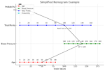
Example 1: data with outliers
Below is an example where we fit the data using linear regression, robust linear regression (Robust against outliers and deviations from normality), quantile regression (Estimates conditional quantiles of the response variable), Theil-sen regression (Computes the median of pairwise slopes between data points) and Local polynomial regression (non-linear relationships and adapts to local variations).

Example 2: data with outliers
- The raw data are 'recovered' from the page Dealing with Outliers Using Three Robust Linear Regression Models.
- ?rlm
- In this case, Theil-sen regression performed better than the other methods.

Choose variables
Stepwise selection of variables
Stepwise selection of variables in regression is Evil
GEE/generalized estimating equations
See Longitudinal data analysis.
Deming regression
Tweedie regression
Model selection, AIC and Tweedie regression
Causal inference
- https://en.wikipedia.org/wiki/Causal_inference
- Visual Guides for Causal Inference including Inverse Probability Weighting.
- Introduction to computational causal inference using reproducible Stata, R, and Python code: A tutorial Smith et Al 2021
- Confounding in causal inference: what is it, and what to do about it?
- An introduction to Causal inference
- Causal Inference cheat sheet for data scientists
- twang package
- The intuition behind inverse probability weighting in causal inference*, Confounding in causal inference: what is it, and what to do about it?
- Outcome [math]\displaystyle{ \begin{align} Y = T*Y(1) + (1-T)*Y(0) \end{align} }[/math]
- Causal effect (unobserved) [math]\displaystyle{
\begin{align}
\tau = E(Y(1) -Y(0))
\end{align}
}[/math]
Inverse-probability weighting removes confounding by creating a “pseudo-population” in which the treatment is independent of the measured confounders... Add a larger weight to the individuals who are underrepresented in the sample and a lower weight to those who are over-represented... propensity score P(T=1|X), logistic regression, stabilized weights. - A Crash Course in Causality: Inferring Causal Effects from Observational Data (Coursera) which includes Inverse Probability of Treatment Weighting (IPTW). R packages used: tableone, ipw, sandwich, survey.
- Propensity score matching
- MatchIt - Nonparametric Preprocessing for Parametric Causal Inference (R package).
- Practical Propensity Score Methods Using R (online book)
- Comparison of Propensity Score Methods and Covariate Adjustment: Evaluation in 4 Cardiovascular Studies Stuart Pocock 2017
- Simple examples to understand what confounders, colliders, mediators, and moderators are and how to “control for” variables in R with regression and propensity-score matching
- Statistical Rethinking (2022 Edition) by Richard McElreath. Youtube.
- Regression and Other Stores (book)
- Riddle: Estimate effect of x on y if you only have two noisy measures of x
- Assignment-Control Plots: A Visual Companion for Causal Inference Study Design, The American Statistician
- Regression and Causality by Michael Schomaker
- A Complete Guide to Causal Inference A compilation of the issues that you kept skipping over, and how to do it right.
- Estimation and Inference of Heterogeneous Treatment Effects using Random Forests Wager Athey 2018. causalTree package.
- generalized random forests CRAN. Athey, Wager, Tibshirani. 2019
- Modeling Heterogeneous Treatment Effects with R (video)
- Causal inference with count regression
- Introduction to structural causal modelling Christopher J. Brown
- Exploring propensity score matching and weighting
- Propensity Score Matching for Causal Inference: Creating Data Visualizations to Assess Covariate Balance in R
Causal Inference in R
Mendelian Randomization
- https://en.wikipedia.org/wiki/Mendelian_randomization
- Github: MR BACOn - A Shiny application for Mendelian Randomization analysis of Biomarker Associations for Causality with Outcomes
- The causal relationship between CSF metabolites and GBM: a two-sample mendelian randomization analysis
- https://github.com/MRCIEU/TwoSampleMR
- Seemingly unrelated regressions from wikipedia
- Advantages: The SUR model is useful when the error terms of the regression equations are correlated with each other. In this case, the ordinary least squares (OLS) estimator is inefficient and inconsistent. The SUR model can provide more efficient and consistent estimates of the regression coefficients
- Disadvantages: One disadvantage of using the SUR model is that it requires the assumption that the error terms are correlated across equations. If this assumption is not met, then the SUR model may not provide more efficient estimates than estimating each equation separately1. Another disadvantage of using the SUR model is that it can be computationally intensive and may require more time to estimate than estimating each equation separately
- Seemingly Unrelated Regression (SUR/SURE)
- How can I perform seemingly unrelated regression in R?
- systemfit package
- spsur package
- Equations for the simplest case:
- [math]\displaystyle{ \begin{align} y_1 &= b_1x_1 + b_2x_2 + u_1 \\ y_2 &= b_3x_1 + b_4x_2 + u_2 \end{align} }[/math]